Sampling, Sample Size, and Particpant Selection
Learning Objectives
In this chapter you will:
- understand the differences between non-probability and probability sampling
- understand the reasons qualitative research has far fewer participants than quantitative research
- discover and understand how to employ a formula to calculate sample size for quantitative research
- discover the best way to obtain participants for your research.
10.1 Sampling
When undertaking research, it is not possible, unless you are conducting the census, to obtain data from the whole population under consideration. Therefore, you collect data from a representative sample of the population targeted in the study. The size of the sample depends on the type of research you are undertaking. Calculating the size of a sample is discussed later in this chapter.
Population Versus Sampling
A sample is a subset of the population we are interested in. Sampling is the process of selecting a subset of the population of interest. A target population is the group of people, objects, or events that you want to study. Remember the target population does not have to be just people.
You start with the population (everyone) which you are not going to be able to access unless you are the government conducting a census. Then we come to the target population, they are those (people, objects, events) the target of your study. Then we have the sample, the portion of the target population that can be accessed or is selectable (Figure 10.1).
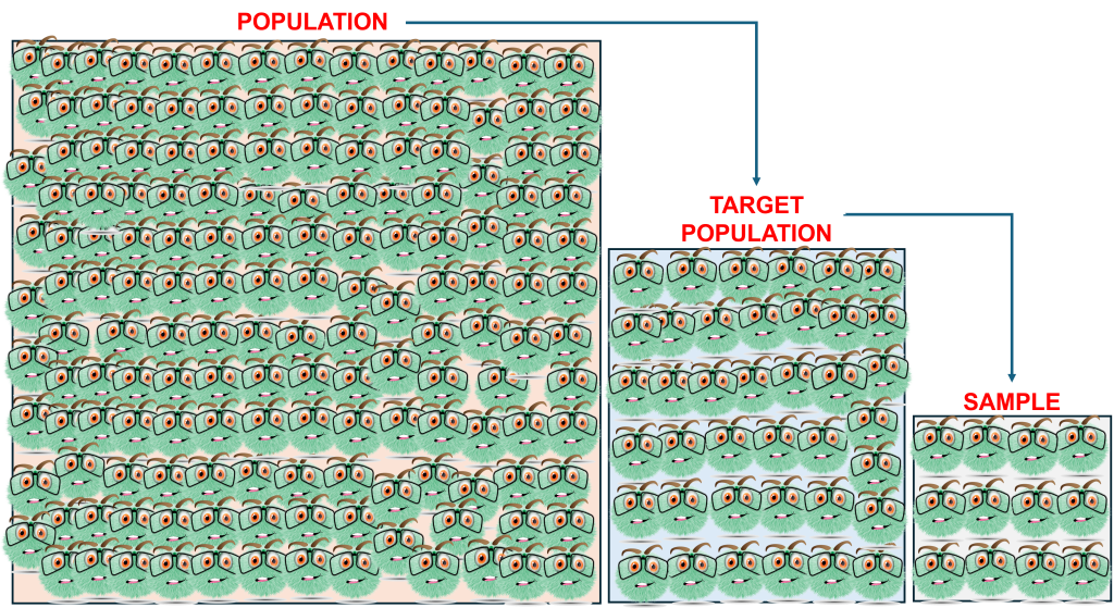
The sample size is determined by the population highlighted in the research question(s) and objectives. Qualitative sampling is purposive, while quantitative sampling needs to support inferential statistics.
Inclusion/Exclusion Criteria
Inclusion and exclusion criteria for participants in research depend largely on the research question(s) and the target population. Inclusion criteria may be on age, for example, the target population are those who fall in the category of Gen Z, therefore those who do not fall in that generational age group are excluded from the study. Your research may require participants to fit several categories to be included in your study, such as age, visitor to the area, length of stay, mode of transport, etc. Inclusion and exclusion criteria are determined once your research topic and question(s) are decided.
Researcher(s) must always be aware of sample selection bias. This can occur for several reasons, such as, one or more sections of the population being over- or under-represented in the sample; an incorrect sampling frame has been used, or is not appropriate, or has insufficient coverage; the data are old, or out-of-date, or the location of data collection is not right. Another bias that can occur is self-selection bias, this occurs when only people with certain characteristics provide information, and non-responsive bias restricts sampling criteria.
Sampling Methods
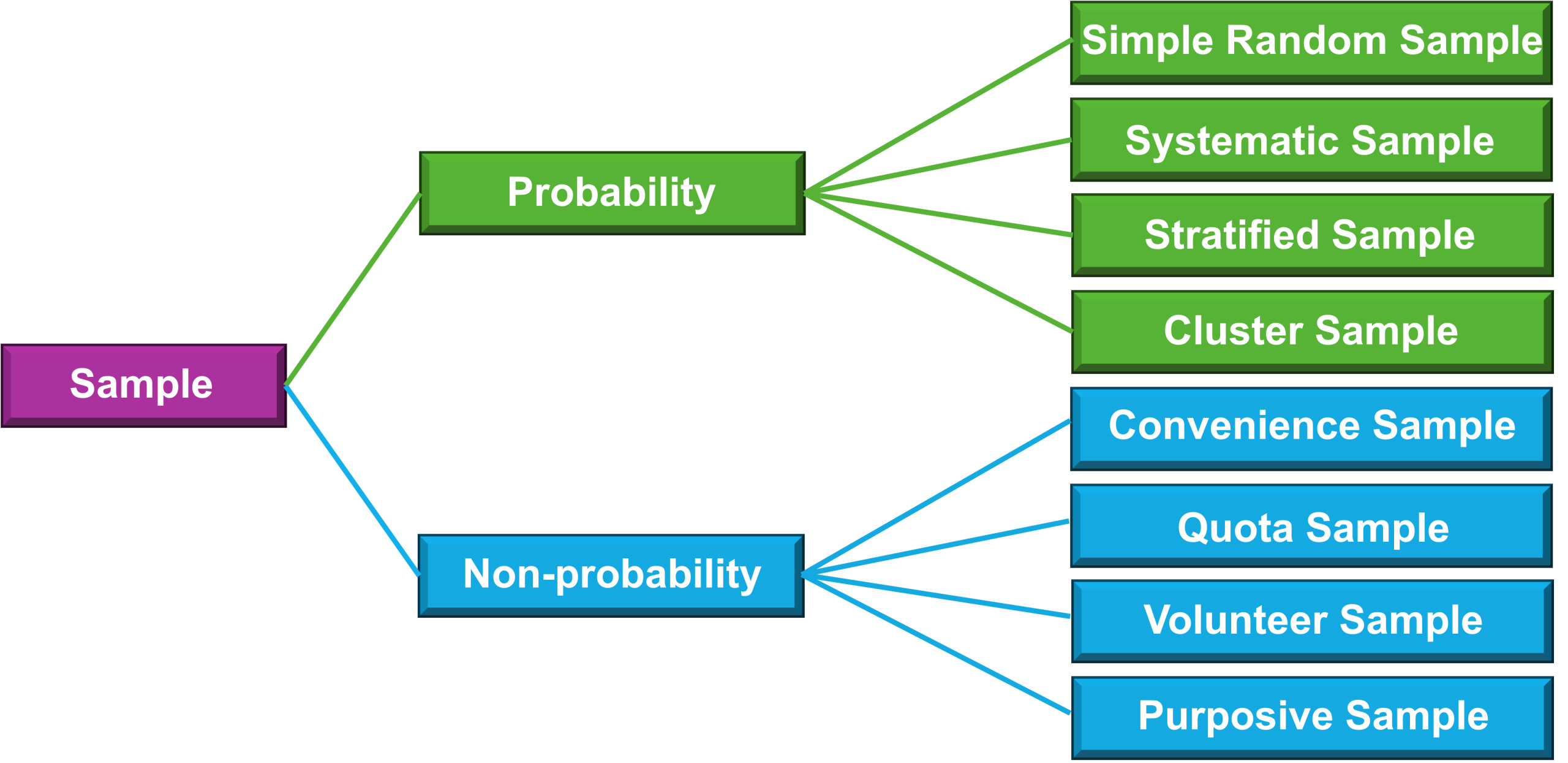
Probability Sampling Versus Non-Probability Sampling
A probability sample is what all researchers aim for. To obtain this type of sample you need to know the exact size of the population, be able to identify every individual within that population, the target population must be completely accessible, and every element in the target population must have a known and equal chance of being selected. Non-probability sampling is more common, but less robust than probability sampling, hence the statistical data is more conservative. Specific probability and non-probability sampling techniques (Figure 10.2) are discussed in the following sections.
Probability Sampling
Simple Random Sample
When using a simple random sample, each unit of a population has the same probability of being selected. Where ‘n’ is the sample size, each combination of ‘n’ elements has the same probability of being selected. An example of this is Saturday Night Lotto (in Australia), there are 45 balls, a total of 8 balls are randomly selected (6 winning, and 2 supplementary) from the lottery machine. All the balls, and all combinations of the balls, have the same a priori probability of being selected. In this case, the lottery machine which contains the 45 balls functions as the sampling frame (Sallis et al., 2021).
In ‘real-life’ it is quite difficult to find a perfect sampling frame that lists or covers all units in a population. Meaning the classic process of drawing a simple random sample where the population units are numbered from 1 to ‘n’, and a random selection of units is sampled from the population is rare. An alternative is to try to select units that as closely as possible represent the population.
Systematic Sample
With systematic sampling, you select every nth unit in your population beginning with a randomly selected unit between 1 and ‘n’. For example:
- You want a sample size of 55 households from a local suburb of 774.
- You might sample every 9th house starting with randomly selected or generated number from 1 to 9.
- The random number is 5, then houses numbered 5, 14, 23, 32, 41, 50… and so on until 55 households were sampled.
- However, you must be aware that systematic bias may occur. This can occur, for example, when every 9th house is in the same position in a street.
If you were investigating traffic noise and every 9th house was a corner house they would be getting traffic noise from two sides. This doubling of the traffic noise may bias your results towards the noise from traffic being greater than those households facing only one road. Therefore, your conclusions on traffic noise in that suburb may not be correct (Sekaran & Bougie, 2013).
Stratified Sample
Stratified sampling is used when the researcher has a variable of interest, and it has been determined that there are subgroup units within the population that are expected to have different parameters on that variable. In this instance, subgroups are generally called ‘stratum’ (singular) or ‘strata’ (plural).
To proceed:
- Divide the population into mutually exclusive, collectively exhaustive strata.
- These strata must be relevant, appropriate, and meaningful to the study’s context.
- Take a simple random sample from each stratum.
- Sample size in each stratum may vary depending on the homogeneity of each stratum.
- Higher levels of homogeneity within a population, the smaller the sample size needed.
Stratified sampling ensures specific subgroups within a population are represented, and certain variables are sufficiently measured. This is useful when heterogeneous subgroups are to be represented, and when each subgroup is homogenous for the variables to be measured. When there is homogeneity within a subgroup fewer units need to be selected. This means weighting can be applied to each subgroup to ensure specific variables are properly represented at the population level (Sallis et al., 2021; Sekaran & Bougie, 2013).
Example using an imaginary scenario:
-
How many flat white coffees do students in the undergraduate statistics subject drink, on average in one week?
- Assume 45% of these students take the subject as an elective.
- The information already obtained says students who take statistics as an elective drink fewer flat whites, on average, in one week, than those who have statistics as a ‘core’ subject.
- Divide the population into 2 strata: ‘elective’ and ‘core’ students.
- Conduct a simple random sample within each stratum.
- This provides an estimate of average flat white consumption of elective, and core statistics subject takers respectively.
- Next, calculate the average consumption for the population by weighting the results of the two strata.
- If the estimate for students where statistics is a core subject is 8 flat whites per week, and the estimate for students where statistics is an elective is 3 flat whites per week, the calculation is as follows: (8 x 0.55) + (3 x 0.45) = (4.4) + (1.35) = 5.75
- From the weighted calculations the population average drinks 5.75 flat whites per week. However, you would generally round this number to six (6).
Note: Be aware that as stratification can take place over several stages, it can become quite complex, on occasion even requiring a ‘masterplan’ to keep track (Sallis et al., 2021).
Cluster Sample
Cluster random sampling:
- Divide a larger population into smaller groups or clusters.
- Then, randomly select clusters to form your sample.
- Is generally used for quite large populations.
- Sample size is also quite large.
- When population, and therefore sample size is too large to study successfully, cluster sampling is used to reduce the total number of participants.
- Occasionally pre-existing groups may be used as clusters, for example, schools, households, towns/cities etc (Simkus, 2023).
Area Cluster Sampling
- Consists of geographic regions (areas), which can be council areas, suburbs, or specified areas of a state (e.g., Far North Queensland)
- If you are surveying residents of a suburb, you would obtain a map of the area, take a sample of streets within the suburb, and select households within each street.
- This can be relatively inexpensive and does not depend on a sampling frame as you already have the map.
Single-Stage Cluster Sampling
- The population is divided into a pre-determined number of clusters.
- The required number of clusters to be sampled are randomly chosen.
- Each element/unit in each selected cluster is investigated.
Double-Stage Cluster Sampling
- Clusters are selected, then data are only obtained from a random sub-sample of individual elements/units within each of the selected clusters.
- Not as accurate as single-stage cluster sampling.
- Generally used only when the cost of testing the entire cluster is prohibitive, or testing the entire cluster is too challenging.
Multi-Stage Cluster Sampling
- It is undertaken in several stages.
- For example, you may have selected urban, regional and rural geographical locations for your study.
- Next, you select specific areas within each location.
- Then you might select primary schools within each selected area.
- You keep going until you have the final clusters of sample elements/units.
- You then sample every element/unit of the final selected clusters (Sekaran & Bougie, 2013; Simkus, 2023).
Non-Probability Sampling
Quota Sampling
Quota sampling is a non-random, convenience method and often used as an alternative to probability sampling as part of a strategy for internet and/or interviewer completed questionnaires. Results from research using quota sampling cannot be generalised to the wider population.
Quota sampling is achieved by:
- Dividing the population into sub-groups.
- All sub-groups must be mutually exclusive.
- Sub-groups are in the same proportion as the population.
- Convenience sample taken from each sub-group.
- Relationship comparisons between selected sub-groups can be tested (Futri et al., 2022; Stratton, 2019).
Purposive Sampling
With purposive sampling researchers select participants that are knowledgeable and/or experienced in relation to the research question/phenomena. These participants must be available and agreeable to participating in the study (Stratton, 2019).
Some of the most common purposive sampling designs are:
Deviant Sampling
- often used in programs to improve processes
- subjects/cases chosen in anticipation of discovering information not commonly available, and that may demonstrate good/problematic findings.
Homogeneous (AKA Dominant) Sampling
- can be used to form focus groups
- participants are chosen to form a sample group where there are similar, dominant characteristics present in relation to the phenomena of interest.
Case Sampling
- The researcher(s) choose cases from a group that have similar characteristics.
- There is no randomisation involved.
- Does not involve all available cases.
- Commonly used with medical cases, for example, medical cases are selected by the researcher for data extraction when they have one or more diagnostic codes that are the same.
Sequential (AKA Consecutive) Sampling
- often used in qualitative studies in developing themes
- sequential subjects/cases are included in the study until no new themes/information emerge
- once no new themes/information emerge, it is said the study has reached ‘saturation point’
- randomisation is not used in selection of participants; therefore, any sampling error is impossible to determine.
Theoretical Sampling
- Research objectives are developed.
- A group is identified to be interviewed in relation to the research question(s).
- Interview criteria are pre-established.
- Researcher(s) analyse the information obtained.
- A second group is selected.
- This second group is interviewed about the findings from the first group.
- The second group may or may not confirm findings of the first group.
- To refine the study, the findings from the first two groups are combined, and a third group is selected.
- This process continues until saturation point is reached.
- This may lead to sample error that cannot be measured. (Stratton, 2019)
Convenience Sample
Convenience sampling is just that, it is the most convenient and easy way to reach potential participants for a study.
For example:
- The Researcher(s) are employed at a university.
- The research population are those aged 18 to 30 who have a smartphone.
- The researcher(s) send emails to all university students aged 18 to 30 asking them if they would participate in a study and providing a link to the survey.
- Even when potential participants do complete the survey, they cannot be said to be a statistically representative sample of the population.
- In this example, all participants are aged 18 to 30 and own smartphones; however, they are not representative of the whole population of those aged 18 to 30 who own smartphones.
Convenience sampling is often used when time constraints are an issue. Results from studies using convenience sampling cannot be generalised to the wider population.
Volunteer Sample
There are 2 techniques for volunteer sampling: Snowball and self-selection:
Snowball Sampling
- It is a continuous referral method.
- Requires research participants to have the same characteristics.
- Researcher(s) recruit an initially limited number of participants.
- In some instances, these first recruits receive a small incentive to recruit other participants for the study.
- These initial participants recruit other participants from family, friends, members of their social groups, members of their sporting clubs etc., these participants then go on to recruit other participants, who recruit other participants… and so on.
- The final participants recruited may have no connection to the initial participants other than the same characteristics under investigation.
- This may be used when the research is focused on hard-to-reach or vulnerable communities. (Valerio et al., 2016)
Self-Selection
- Participants nominate themselves to participate in a survey or similar research.
- Participants volunteer as they have an interest in what is being studied.
- Their interest in the topic may be at the extremes of positive and negative opinions, therefore any average view on the topic is hidden.
- This means there is a high possibility that the results from the sample are biased.
- If using a questionnaire, self-selection sampling can be achieved by leaving the questionnaires in a range of locations appropriate to the topic under study.
- Other means of recruitment may be achieved by using posters or flyers which provide researcher contact information, a QR code can make this easier for potential participants.
- Web pages or posts (where platforms permit) can encourage people to self-select and complete online surveys (Galloway, 2005).
10.2 Sample Size and Participant Selection
Qualitative Research
For qualitative research using interviews or observations, a researcher generally targets a sample size between 10 and 40. However, this all depends on the process you have selected and the target population. Then you keep sampling until theoretical saturation, that is, continue sampling and data collection, and analysis, until no new conceptual insights are generated.
When focus groups are used, the target number for each group is generally 8 to 12. This provides the best balance of productive interaction against managing the interaction effectively. The number of focus groups required depends on the research question(s) and objectives. But you do need the same number of members in each focus group for that specific study.
Quantitative Research
Remember, in quantitative research, a sample is used as a substitute for the population. The sample should be free of sample selection bias and be large enough for the researcher(s) to be confident any number that describes the sample (sample statistics) is precise enough to be useful to the actual population number (parameter). This is based on probability laws in mathematics where the odds are calculated that any given sample mean is likely to be the actual population mean (confidence). The idea is that if the exact same research was done repeatedly, with different samples from the same population, the mean of the sample means should equal the population mean.
When deciding on the sample size a researcher must consider costs, if the sample is too big, or too small the data collection is just a waste of money and time. A researcher when considering sample size must consider, and allow, for non-responses and incomplete responses; how many subgroups have to be accurately described? Generally, it is a balancing act between precision and accuracy.
With a survey, to increase representativeness, precision, and confidence, a larger sample size is required. If the researcher does not need to describe subgroups or test for any differences, in Table 10.1, the confidence level is 95%. Look down the ‘N’ column for your population size (nearest to it), then look across the row to your margin of error (5%, 3%, 2%, 1%) to find the required sample size. If you Google “sample size with margin of error table”, you get multiple examples under ‘images’.
Table 10.1. Population with sample size for margins of error at 95% confidence level (N=population) (sample sizes were calculated with Qualtrics’ sample size calculator)
| Sample Size with Margin of Error | Sample Size with Margin of Error | |||||||||
| N | 5% | 3% | 2% | 1% | N | 5% | 3% | 2% | 1% | |
| 10 | 10 | 10 | 10 | 10 | 440 | 206 | 312 | 372 | 421 | |
| 15 | 15 | 15 | 15 | 15 | 460 | 210 | 322 | 387 | 439 | |
| 20 | 20 | 20 | 20 | 20 | 480 | 214 | 332 | 401 | 458 | |
| 25 | 24 | 25 | 25 | 25 | 500 | 218 | 341 | 414 | 476 | |
| 30 | 28 | 30 | 30 | 30 | 550 | 227 | 363 | 448 | 521 | |
| 35 | 33 | 34 | 25 | 35 | 600 | 235 | 385 | 481 | 565 | |
| 40 | 37 | 39 | 40 | 40 | 650 | 242 | 404 | 512 | 609 | |
| 45 | 41 | 44 | 45 | 45 | 700 | 249 | 423 | 542 | 653 | |
| 50 | 45 | 48 | 49 | 50 | 750 | 255 | 441 | 572 | 696 | |
| 55 | 49 | 53 | 54 | 55 | 800 | 260 | 458 | 601 | 739 | |
| 60 | 52 | 57 | 59 | 60 | 850 | 265 | 474 | 628 | 781 | |
| 65 | 56 | 62 | 64 | 65 | 900 | 270 | 489 | 655 | 823 | |
| 70 | 60 | 66 | 69 | 70 | 950 | 274 | 503 | 681 | 865 | |
| 75 | 63 | 71 | 73 | 75 | 1000 | 278 | 517 | 706 | 906 | |
| 80 | 67 | 75 | 78 | 80 | 1100 | 285 | 542 | 755 | 987 | |
| 85 | 70 | 79 | 83 | 85 | 1200 | 291 | 565 | 801 | 1067 | |
| 90 | 73 | 83 | 87 | 90 | 1300 | 297 | 587 | 844 | 1145 | |
| 95 | 77 | 88 | 92 | 95 | 1400 | 302 | 606 | 885 | 1222 | |
| 100 | 80 | 92 | 97 | 99 | 1500 | 306 | 624 | 924 | 1298 | |
| 110 | 86 | 100 | 106 | 109 | 1600 | 310 | 641 | 961 | 1372 | |
| 120 | 92 | 108 | 115 | 119 | 1700 | 314 | 656 | 996 | 1445 | |
| 130 | 98 | 116 | 124 | 129 | 1800 | 317 | 670 | 1029 | 1516 | |
| 140 | 103 | 124 | 133 | 138 | 1900 | 320 | 684 | 1061 | 1587 | |
| 150 | 108 | 132 | 142 | 148 | 2000 | 323 | 696 | 1092 | 1656 | |
| 160 | 113 | 140 | 151 | 158 | 2200 | 328 | 719 | 1148 | 1790 | |
| 170 | 118 | 147 | 159 | 168 | 2400 | 332 | 739 | 1201 | 1921 | |
| 180 | 123 | 155 | 168 | 177 | 2600 | 335 | 757 | 1249 | 2047 | |
| 190 | 128 | 162 | 177 | 187 | 2800 | 338 | 773 | 1293 | 2168 | |
| 200 | 132 | 169 | 185 | 196 | 3000 | 341 | 788 | 1334 | 2286 | |
| 210 | 136 | 176 | 194 | 206 | 3500 | 347 | 818 | 1424 | 2566 | |
| 220 | 140 | 183 | 202 | 216 | 4000 | 351 | 843 | 1501 | 2824 | |
| 230 | 144 | 190 | 210 | 225 | 4500 | 354 | 863 | 1566 | 3065 | |
Quantitative Sample Size Formula
The manual formula for calculating a quantitative sample size is as follows:
- your confidence level is 95%
- your margin of error is 5% = 0.05
- when the confidence level is 95% the constant used in the formula is 1.96
- when the confidence level is 90% the constant used is 1.64; for 99% it is 2.58
- 0.5 is a conservative estimate of how many subjects have the characteristics being measured; this can be viewed as a constant.
Example: margin of error = 5% = 0.05, confidence level = 95%

In Figure 10.3, this is a minimum sample size where the margin of error is 5%, the total is rounded to 385. This example is a general survey where the researcher(s) want to be 95% confident with their results and are prepared to live with 5% error; therefore this formula can be used to determine at least 385 subjects are required in the sample. The final formula is rounding 0.9604 to a whole number, one (1), which then provides an approximate sample size of 400. Research suggests that even if there is allowance for non-response error there should still be at least a 60% response rate.
When the margin of error is changed to 3% (0.03) (Figure 10.4) and the confidence level is 95%, a larger sample size is required. The finer the margin of error, the larger the sample size required.

Response Rate
The response rate for surveys can vary greatly, but the researcher should have a response rate exceeding 50%. A quick, easy-to-understand example of how to work out a response rate of 80% is for example, a researcher asks 100 people to undertake their survey, and 80 people actually complete the survey. The response rate is therefore 80%.
Figure 10.5a calculates a survey sample size when the base sample size has been calculated at 385 (Figure 21.3), and the response rate required is 80%. The new sample size required is 482.

Using the base sample size from Figure 10.4 of 1,068, and a response rate of 80% the new sample size required is 1,335 (Figure 10.5b).

Now, what if you expect a lower response rate, say 65%. We plug this into our formula along with our base sample size (Figure 10.3) of 385 for an updated sample size requirement of 593 (Figure 10.6).

We go back to Figure 10.4, the margin of error is 3% and the confidence level is 95%, the formula provided a base sample size of 1,068. We plug this into the formula and calculate the new required sample size at a response rate of 65% is 1,644 (Figure 10.7).

Key Takeaways
-
Non-probability sampling is more common, but less robust than probability sampling; hence, the statistical data is more conservative.
- Probability sampling and non-probability sampling are generally used separately, but can be used together.
- Qualitative research has fewer participants than quantitative research.
- Qualitative research generally uses small groups of participants or multiple small groups of participants.
- To determine survey sample size for quantitative research, there are specific formulas to use.
- The formulas require a margin of error and confidence level for the initial calculations.
- Once you have a base sample size, you decide on a response rate, for example, 80% or 65%. The response rate, along with the base sample size figure, are plugged into the response rate formula to provide an updated sample size figure.
- All response rates should exceed 50%.
References
Futri, I. N., Risfandy, T., & Ibrahim, M. H. (2022). Quota sampling method in online household surveys. MethodsX, 9, Article 101877. https://doi.org/10.1016/j.mex.2022.101877
Galloway, A. (2005). Non-probability sampling. In K. Kempf-Leonard (Ed.). Encyclopedia of social measurement (Vol. 2, pp. 859-864). Elsevier. https://doi.org/10.1016/BO-12-369398-5/00382-0
Martelli, J., & Greener, S. (2018). An Introduction to business research methods (3rd ed.). Bookboon. https://bookboon.com/en/an-introduction-to-business-research-methods-ebook
Sallis, J. E., Gripsrud, G., Olsson, U. H., & Silkoset, R. (2021). Research methods and data analysis for business decisions: A primer using SPSS. Springer.
Sekaran, U. & Bougie, R. (2013). Research methods for business: A skill building approach (6th ed.). Wiley.
Simkus, J. (2023, July 31). Cluster sampling: Definition, method, and examples. Simply Psychology. https://www.simplypsychology.org/cluster-sampling.html
Stratton, S. J. (2019). Data sampling strategies for disaster and emergency health research. Prehospital and Disaster Medicine, 34(3), 227-230. https://doi.org/10.1017/S1049023X19004412
Valerio, M. A., Rodriguez, N., Winkler, P., Lopez, J., Dennison, M., Liang, Y., & Turner, B. J. (2016). Comparing two sampling methods to engage hard-to-reach communities in research priority setting. BMC Medical Research Methodology, 16, 2-11. https://doi.org/10.1186/s12874-016-0242-z
