9.4. Correlational Research
By Rajiv S. Jhangiani, I-Chant A. Chiang, Carrie Cuttler and Dana C. Leighton, adapted by Marc Chao and Muhamad Alif Bin Ibrahim
Correlational research is a type of non-experimental study where researchers measure two variables (either binary or continuous) and analyse the statistical relationship between them, known as a correlation. In this type of research, there is little to no control over extraneous variables.
Researchers often choose correlational research when their goal is to describe and predict relationships between variables rather than establish causation. For example, if two variables are correlated, researchers can use regression analysis to predict one variable based on the other. This approach aligns with two primary goals of science: to describe phenomena and to make predictions about future outcomes.
In some cases, correlational research is preferred because manipulating an independent variable might be impossible, impractical, or unethical. For instance, studying the relationship between cannabis use frequency and memory performance cannot ethically involve manipulating how often people use cannabis. Instead, researchers measure both variables and analyse the correlation to understand their relationship without direct intervention.
Another significant advantage of correlational research is its role in establishing reliability and validity for measurement tools. For example, if a researcher develops a short extraversion questionnaire, they can compare it with a longer, well-established version. A strong correlation between the two sets of scores would suggest that the shorter test is valid and reliable.
Correlational studies also tend to have higher external validity compared to experiments. While experiments excel at internal validity through tight control over variables, they often create artificial conditions that might not exist in the real world. In contrast, correlational research is typically conducted in more natural settings, making its findings more generalisable to everyday situations.
Additionally, correlational research can complement experimental findings, providing converging evidence to strengthen a theory. When an experimental study demonstrates causation and a correlational study supports the same relationship in a natural context, researchers can have greater confidence in the theory’s validity. For example, studies showing a correlation between watching violent television and aggressive behaviour have been reinforced by experiments that establish a causal connection (Bushman & Huesmann, 2011).
Does Correlational Research Always Involve Quantitative Variables?
A common misunderstanding among new researchers is the belief that correlational research must always involve two quantitative variables, such as scores from personality tests or the number of daily stressors and symptoms someone experiences. However, what truly defines correlational research is not the type of variables used, but rather the method of data collection, specifically, that both variables are measured and not manipulated. This principle holds true whether the variables are quantitative (e.g., test scores) or categorical (e.g., nationality or occupation).
For example, consider a study where a researcher administers the Rosenberg Self-Esteem Scale to 50 American college students and 50 Japanese college students. At first glance, this might seem like a between-subjects experiment, but it is actually correlational research because the researcher did not actively manipulate nationality; it was simply measured. Similarly, in the study by Cacioppo and Petty comparing college faculty and factory workers on their need for cognition, the research was correlational because participants’ occupations were not manipulated, only observed.
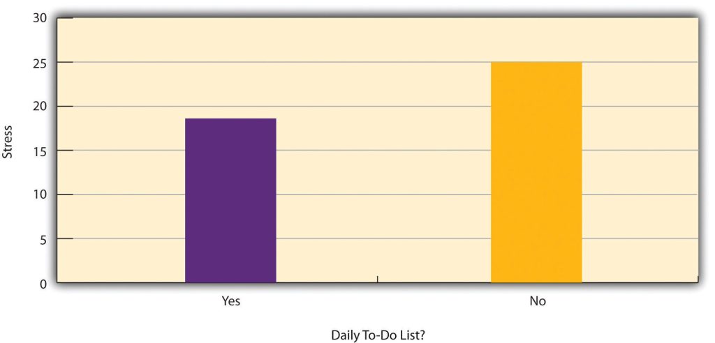
To clarify this distinction, consider a hypothetical study investigating the relationship between making daily to-do lists and stress levels, such as the one shown in Figure 9.4.1. Whether this study is classified as correlational or experimental depends entirely on how it was conducted.
- If participants were randomly assigned to either make daily to-do lists or not make them, then this would be an experiment. In this case, researchers could make a causal claim, such as concluding that making daily to-do lists reduces stress.
- On the other hand, if participants were simply asked whether they usually make daily to-do lists, it would be a correlational study. In this scenario, researchers could only identify a statistical relationship between the two variables. They could not determine whether stress reduces people’s ability to plan ahead (the directionality problem) or whether a third variable, such as conscientiousness, influences both stress levels and the likelihood of making to-do lists (the third-variable problem).
Data Collection in Correlational Research
In correlational research, the key feature is that neither variable is manipulated by the researcher. What matters is that both variables are measured as they naturally occur, not how or where the data collection happens.
For example, a researcher might invite participants into a laboratory to complete a computerised backward digit span task (to measure memory) and a risky decision-making task (to measure risk tolerance). They could then analyse the relationship between the scores on these two tasks.
Alternatively, another researcher might visit a shopping mall and ask people about their attitudes toward the environment and their shopping habits. They would then assess the relationship between these two variables.
In both examples, even though the settings and data collection methods differ, the studies are still considered correlational because no variable was manipulated, they were only measured.
Correlations Between Quantitative Variables
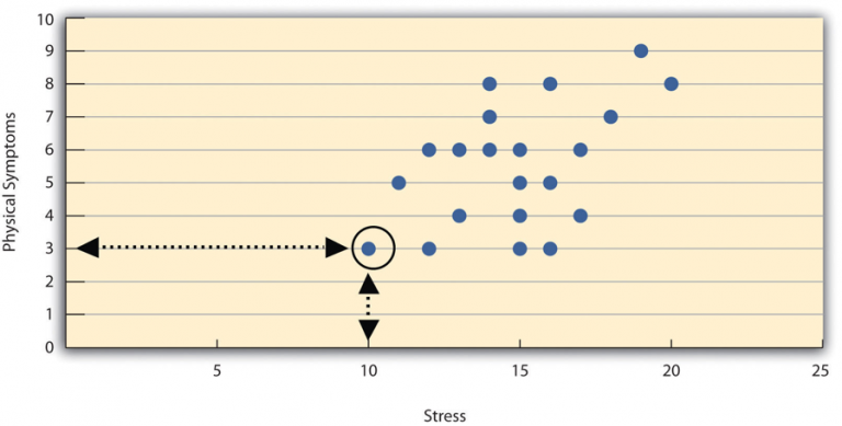
Correlations between quantitative variables are often illustrated using scatterplots. In a scatterplot, each point represents one person’s score on two variables. For example, imagine a study measuring the relationship between stress levels and physical symptoms. A point on the scatterplot might represent a person with a stress score of 10 and three physical symptoms (as shown in Figure 9.4.2). When observing all the points together, a pattern often emerges. If higher stress levels correspond with more physical symptoms, this indicates a positive relationship, as one variable increases, the other tends to increase as well. In contrast, a negative relationship occurs when higher scores on one variable are associated with lower scores on the other. For example, stress levels and immune system functioning typically show a negative relationship, where higher stress is linked to lower immune function.
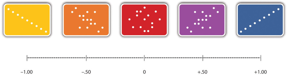
As illustrated in Figure 9.4.3, the strength of this relationship is measured using Pearson’s Correlation Coefficient (r), which ranges from -1.00 to +1.00. A value of +1.00 represents a perfect positive correlation, while -1.00 represents a perfect negative correlation. A value of 0 indicates no relationship between the two variables. In a scatterplot, a correlation near 0 will appear as a random “cloud” of points, while values closer to ±1.00 show points aligning more closely along a straight line. Correlation coefficients around ±0.10 are considered small, around ±0.30 are considered medium, and around ±0.50 are considered large. It is important to note that the sign (+ or -) indicates the direction of the relationship, not its strength. For example, +0.30 and -0.30 represent relationships of equal strength, but one is positive and the other negative.
However, there are two scenarios where Pearson’s r can be misleading:
Nonlinear Relationships
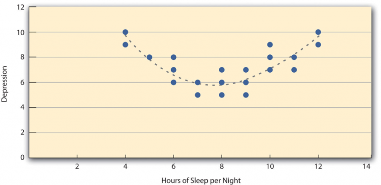
Pearson’s r works well for linear relationships, where the data points align roughly along a straight line. However, it is not suitable for nonlinear relationships, where the best-fit line would be a curve. For example, Figure 9.4.4 illustrates the relationship between sleep duration and depression, forming an upside-down U-shape. This hypothetical data suggests that people who sleep too little or too much may show higher depression levels, while those who sleep around eight hours have the lowest depression levels. Even though there is a strong relationship, Pearson’s r would be close to zero because it does not fit a straight line. This highlights the importance of creating a scatterplot first to visually check if the relationship is linear before relying on Pearson’s r.
Restriction of Range
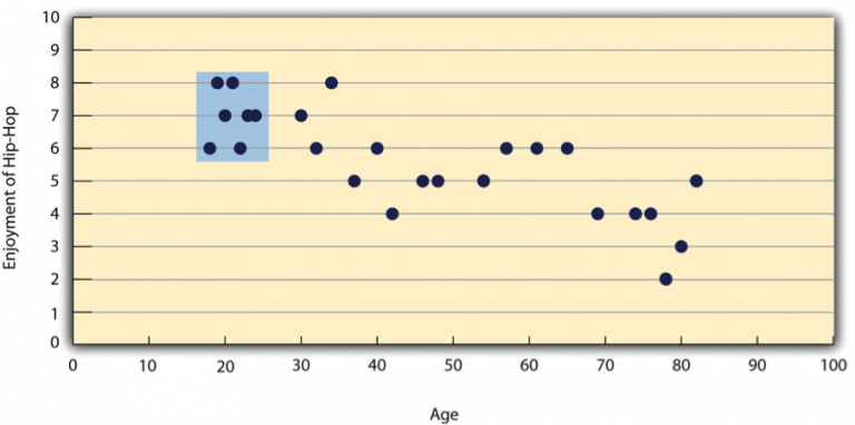
Pearson’s r can also be misleading when there is limited variation in one or both variables. This issue, called restriction of range, occurs when the sample does not represent the full spectrum of values. For instance, imagine a strong negative correlation between age and enjoyment of hip-hop music across a wide range of ages. However, if the sample only includes 18- to 24-year-olds, as shown in the blue box in Figure 9.4.5, the correlation might disappear entirely because this group shows limited variation in music preference. To avoid this, researchers should aim to include a wide range of values for their key variables. If restriction of range happens unintentionally, it is essential to interpret Pearson’s r cautiously and consider statistical adjustments when necessary.
Correlation Does Not Imply Causation
You have likely heard the phrase, “Correlation does not imply causation”. A humorous example comes from a 2012 study showing a strong positive correlation (Pearson’s r = 0.79) between a country’s per capita chocolate consumption and the number of Nobel Prizes awarded to its citizens. While the data suggest a relationship, it is unlikely that eating more chocolate directly causes people to win Nobel Prizes. Recommending parents to give their children more chocolate in hopes of future Nobel success would not make much sense.
There are two key reasons why correlation does not imply causation:
- The Directionality Problem: When two variables (X and Y) are correlated, it could mean that X causes Y, or it could mean that Y causes X. For example, studies often show that people who exercise regularly tend to be happier. While it is tempting to conclude that exercise causes happiness, the reverse could also be true, where happier people might be more inclined to exercise, perhaps because they have more energy or seek social interaction at the gym.
- The Third-Variable Problem: Sometimes, two variables (X and Y) are correlated not because one causes the other, but because a third variable (Z) affects both. For instance, the correlation between chocolate consumption and Nobel Prize wins could actually stem from a third factor, like geographic or economic factors. European countries, for example, often have high chocolate consumption and also invest significantly in education and scientific research. Similarly, the link between exercise and happiness could be explained by a third variable, such as physical health, where healthier people are both more likely to exercise and to feel happier.
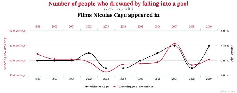
Correlations caused by third variables are often referred to as spurious correlations. These are relationships that appear meaningful but are actually coincidental or driven by an unseen factor.
For more entertaining examples of spurious correlations, you can visit Tyler Vigen’s website, where you will find charts showing amusing and unlikely connections between seemingly unrelated variables, such as the one shown in Figure 9.4.6.
“Lots of Candy Could Lead to Violence” – a Misleading Claim
While psychologists understand that correlation does not imply causation, many journalists often overlook this principle. A website dedicated to exploring this issue, Correlation or Causation?, highlights numerous media reports where headlines suggest a causal relationship when the evidence only shows a correlation. These misunderstandings usually stem from directionality problems or third-variable problems.
One example is a study showing that children who ate candy every day were more likely to be arrested for violent offences later in life. The headline suggested that candy could “lead to” violence. But is this really true? Could there be other explanations for this statistical relationship? Perhaps children who ate more candy also grew up in environments with less parental supervision or had less balanced diets, both of which could contribute to behavioural issues. A more accurate headline might say, “Study Finds Link Between Daily Candy Consumption and Later Behavioural Problems,” instead of implying direct causation.
Addressing the Directionality and Third-Variable Problems
Researchers use specific strategies to address these issues, and the most effective approach is to conduct an experiment. For example, rather than just measuring how much people exercise, a researcher might randomly assign participants to either run on a treadmill for 15 minutes or sit on a couch for 15 minutes.
This minor change in the research design is incredibly powerful. If the participants who exercised show improved moods compared to those who did not, the causal link becomes clearer. This is because:
- The directionality problem is eliminated, since mood cannot influence exercise levels because the researcher controlled who exercised and who did not.
- The third-variable problem is minimised, since factors like physical health or energy levels cannot explain the mood difference since random assignment balanced those variables across the groups.
Assessing Relationships Among Multiple Variables
In correlational research, psychologists often measure multiple variables, whether binary (e.g., yes/no) or continuous (e.g., numerical scores), to understand the statistical relationships among them. For example, Nathan Radcliffe and William Klein conducted a study on middle-aged adults to explore how optimism (measured using the Life Orientation Test) is related to factors associated with heart attack risks. These factors included participants’ overall health, their knowledge of heart attack risk factors, and their perceptions of their own heart attack risk. The researchers found that more optimistic individuals tended to exercise more, had lower blood pressure, were more informed about heart attack risk factors, and accurately perceived their risk as lower than that of their peers.
Another study by Ernest Jouriles and colleagues examined the relationship between adolescents’ experiences of physical and psychological aggression in relationships and their levels of psychological distress. Since measures of physical aggression often produce skewed results, the researchers converted the data into binary categories (0 = did not occur, 1 = did occur). They did the same for psychological aggression and then analysed the relationships between these variables. The results revealed that adolescents who experienced physical aggression were also moderately likely to experience psychological aggression, and those exposed to psychological aggression reported higher psychological distress.
This approach is also frequently used to validate new psychological measures. For instance, when John Cacioppo and Richard Petty developed the Need for Cognition Scale (a tool measuring how much people enjoy and value thinking), they tested it on a large sample of college students. They also measured intelligence, socially desirable responding (the tendency to give what one believes is the “right” or socially acceptable answer), and dogmatism. As shown in Table 9.4.1, the findings were presented in a correlation matrix showing statistical relationships (Pearson’s r) between each pair of variables. For example, the correlation between need for cognition and intelligence was +.39, while the correlation between intelligence and socially desirable responding was +.02.
The overall pattern of correlations supported the researchers’ expectations about how need for cognition scores should relate to these other psychological constructs.
| Need for cognition | Intelligence | Social desirability | Dogmatism | |
| Need for cognition | — | |||
| Intelligence | +.39 | — | ||
| Social desirability | +.08 | +.02 | — | |
| Dogmatism | −.27 | −.23 | +.03 | — |
Factor Analysis
Factor analysis is a statistical method used to identify patterns among a large set of related variables. It works by grouping these variables into smaller clusters, where variables within each cluster are strongly correlated with one another but show weaker correlations with variables in other clusters. Each cluster represents an underlying concept or “factor” that captures the shared characteristics of the variables within it.
For example, when people are tested on various mental tasks, factor analysis often reveals two primary factors: one associated with mathematical intelligence (tasks like arithmetic, quantitative estimation, and spatial reasoning) and the other with verbal intelligence (tasks like grammar, reading comprehension, and vocabulary). Similarly, the Big Five personality traits, such as extraversion, openness, and conscientiousness, were identified through factor analysis by grouping specific traits that tend to co-occur.
Another interesting application of factor analysis comes from research by Peter Rentfrow and Samuel Gosling. They asked over 1,700 university students to rate their preferences across 14 music genres. Factor analysis revealed four distinct clusters or dimensions of musical preference:
- Reflective and Complex: Blues, jazz, classical, and folk music
- Intense and Rebellious: Rock, alternative, and heavy metal music
- Upbeat and Conventional: Country, soundtrack, religious, and pop music
- Energetic and Rhythmic: Rap/hip-hop, soul/funk, and electronica music
These clusters suggest that musical preferences are not random but follow meaningful patterns that reflect broader tastes.
However, it is important to note that factors are not categories. Factor analysis does not classify people into rigid groups. For instance, someone high in extraversion might also score high or low in conscientiousness. Similarly, someone who enjoys reflective and complex music might also like intense and rebellious music. Additionally, factors reveal structure, not meaning. Factor analysis identifies patterns, but it is up to researchers to interpret and label these factors meaningfully. For example, researchers have suggested that the Big Five personality factors arise from different genetic influences.
Exploring Causal Relationships in Correlational Research
While it is true that correlation does not imply causation, correlational research can still offer valuable insights into potential causal relationships between variables. Although it cannot definitively prove that one variable causes another, it can help rule out alternative explanations using a technique called partial correlation. Instead of controlling third variables through random assignment or holding them constant (as in experiments), researchers measure these third variables and include them in statistical analyses.
Imagine a researcher investigating whether watching violent television shows leads to aggressive behaviour. She suspects that socioeconomic status (SES) might be a third variable influencing this relationship. To address this, she conducts a study measuring three factors: the amount of violent television participants watch, their aggressive behaviours, and their SES.
First, she calculates the correlation between violent TV viewing and aggression and finds a moderate positive correlation of +0.35. Next, she uses partial correlation to control for SES. This analysis isolates the relationship between violent TV viewing and aggression, removing the influence of SES on both variables.
- If the partial correlation remains high (e.g., +0.34), this suggests that the relationship between violent TV viewing and aggression exists independently of SES. SES is not a driving third variable.
- If the correlation drops significantly (e.g., +0.03), this suggests that SES is likely the key factor driving the relationship.
- If the correlation decreases but remains moderate (e.g., +0.20), this indicates that SES explains part of the relationship, but not all of it.
While partial correlation is a powerful statistical tool for addressing third-variable problems, it has its limitations. It does not resolve the directionality problem (we still don’t know if watching violent TV causes aggression or if aggressive individuals are drawn to violent TV). Additionally, there could be other unmeasured third variables influencing the relationship that were not accounted for in the analysis.
Understanding Regression in Research
Once a relationship between two variables is identified, researchers can use this relationship to predict one variable based on another. For example, if we know there is a correlation between IQ scores and GPA, we can use someone’s IQ score to predict their GPA. While correlation coefficients describe the strength and direction of a relationship, regression analysis goes a step further by providing a statistical model to make predictions.
In a regression analysis, the variable used to make predictions is called the predictor variable, and the variable being predicted is called the outcome variable (or criterion variable). The basic formula for regression looks like this:
Y = 𝑏1𝑋1
- Y represents the predicted score on the outcome variable.
- b1 is the regression weight (slope), which shows how much the outcome variable changes for each one-unit increase in the predictor variable.
- X1 represents the person’s score on the predictor variable.
To predict someone’s score on the outcome variable (Y), you simply multiply their predictor score (X1) by the regression weight (b1).
Simple vs. Multiple Regression
While simple regression involves predicting an outcome using one predictor variable, multiple regression uses several predictor variables (X1, X2, X3,…Xi) to predict an outcome variable (Y). The general formula for multiple regression looks like this:
𝑌 = 𝑏1𝑋1 + 𝑏2𝑋2 + 𝑏3𝑋3 + … + 𝑏i𝑋i
- Each b (e.g., b1, b2) represents how much each predictor variable contributes to predicting the outcome variable.
- The regression weights show how much the outcome variable changes with a one-unit increase in each predictor variable, assuming all other variables remain constant.
Why Use Multiple Regression?
Multiple regression is valuable because it can show how each predictor variable contributes to an outcome variable while statistically controlling for other predictor variables.
For example, imagine a researcher wants to understand how income and health relate to happiness. These two predictors (income and health) are related to each other, making it difficult to tell if one directly influences happiness or if the relationship is indirect.
- If wealthier people are happier, is it because they are healthier?
- If healthier people are happier, is it because they tend to have more money?
Using multiple regression, researchers can statistically control for one variable while examining the other. This means they can isolate the effect of income on happiness, independent of health, and vice versa.
Research using multiple regression has shown that both income and health contribute only slightly to happiness, except in extreme cases of poverty or severe illness (Diener, 2000).
However, while regression analysis is powerful for identifying patterns and predicting outcomes, it cannot definitively establish causation. At best, it reveals patterns of relationships that are consistent with some causal explanations and inconsistent with others. To establish causality, experimental designs remain the gold standard.
References
Bushman, B. J. & Huesmann, L. R. (2011). Effects of violent media on aggression. In D. G. Singer & J. L. Singer (Eds.), Handbook of children and the media (2nd ed., pp. 231-248). Sage.
Cacioppo, J. T., & Petty, R. E. (1982). The need for cognition. Journal of Personality and Social Psychology, 42, 116–131.
Diener, E. (2000). Subjective well-being: The science of happiness and a proposal for a national index. American Psychologist, 55(1), 34–43. https://doi.org/10.1037/0003-066X.55.1.34
Chapter Attribution
Content adapted, with editorial changes, from:
Research methods in psychology, (4th ed.), (2019) by R. S. Jhangiani et al., Kwantlen Polytechnic University, is used under a CC BY-NC-SA licence.
