By Rajiv S. Jhangiani, I-Chant A. Chiang, Carrie Cuttler and Dana C. Leighton, adapted by Marc Chao and Muhamad Alif Bin Ibrahim

The term quasi means “resembling”, so quasi-experimental research is similar to true experimental research but lacks one key element. In a true experiment, random assignment ensures participants are evenly distributed across groups, or counterbalancing helps control order effects in within-subject designs. In quasi-experiments, one of these safeguards is missing. While the researcher manipulates an independent variable, either there is no control group, or participants are not randomly assigned to conditions (Cook & Campbell, 1979).

Quasi-experiments have an advantage over non-experimental research because the independent variable is manipulated before measuring the dependent variable. This eliminates the directionality problem, where it is unclear which variable affects the other. However, because random assignment or counterbalancing is not used, there is still a risk of confounding variables, which are other differences between groups that could explain the results. As a result, quasi-experiments fall somewhere between non-experimental research and true experiments in terms of internal validity.

Quasi-experiments are especially common in real-world field settings, where random assignment is impractical or impossible. They are frequently used to evaluate the effectiveness of treatments, such as a psychotherapy program or an educational intervention.

One-Group Posttest Only Design

In a one-group posttest only design, researchers apply a treatment or manipulation (independent variable) and then measure the dependent variable just once after the treatment. For example, a researcher might introduce an anti-drug education program to elementary school students and then immediately measure their attitudes toward illegal drugs after the program concludes.

This design is considered the weakest type of quasi-experimental design because it lacks a control or comparison group. Without a control group, there is no way to know what the students’ attitudes would have been without the program. Any observed change could be due to other factors, such as natural development, outside influences, or participant expectations.

Despite these limitations, findings from one-group posttest only designs are often widely reported in the media and frequently misinterpreted by the public. For instance, an advertisement might claim that 80% of women noticed brighter skin after using a specific cleanser for a month. However, without a comparison group, it is impossible to know whether the improvement was actually caused by the cleanser or would have happened naturally over time.

One-Group Pretest-Posttest Design

In a one-group pretest-posttest design, researchers measure a dependent variable before and after introducing a treatment or intervention. For example, if a researcher wants to test the effectiveness of an anti-drug education program on elementary school students’ attitudes toward illegal drugs, they might measure the students’ attitudes one week, implement the program the next week, and then measure their attitudes again the following week.

This design is similar to a within-subjects experiment, where participants serve as their own control group. However, unlike a true experiment, there is no counterbalancing of conditions because participants cannot be exposed to the treatment before the control condition.

If students’ attitudes improve after the anti-drug program, it seems logical to credit the program for the change. However, this conclusion is often uncertain because several threats to internal validity can provide alternative explanations for the observed change.

History is one such threat. Events occurring between the pretest and posttest might have influenced participants’ attitudes. For example, a widely broadcast anti-drug message on TV or news of a celebrity’s drug-related death could have affected the students’ views independently of the program.

Maturation is another concern. Over time, participants naturally grow, learn, and develop. If the program lasted a year, improvements in reasoning skills or emotional maturity might explain the change, rather than the program itself.

The act of taking the pretest itself can also affect posttest results, a threat known as testing effects. For instance, completing a survey about drug attitudes might prompt participants to reflect on the topic, leading to changes in their attitudes before the program even begins.

Instrumentation can also undermine validity if the measuring tool changes over time. For example, participants might have been highly attentive during the pretest survey but less focused and engaged during the posttest, leading to inconsistent results.

Another issue is regression to the mean, a statistical phenomenon where individuals who score extremely high or low on one occasion are likely to score closer to the average on subsequent occasions. If participants were selected for the program based on unusually extreme attitudes toward drugs, their posttest scores would likely shift closer to average, regardless of the program’s impact.

Closely related to regression to the mean is spontaneous remission, where medical or psychological problems improve naturally over time without treatment. For instance, people with depression often report improvement even without intervention. Research shows that participants in waitlist control groups for depression treatments tend to improve by 10–15% before receiving any therapy at all (Posternak & Miller, 2001).

Given these threats to internal validity, researchers must be cautious when interpreting results from one-group pretest-posttest designs. A common way to address these concerns is to add a control group, which is a group of participants who do not receive the treatment. Both groups would be subject to the same threats (e.g., history, maturation, testing effects), allowing researchers to more accurately measure the treatment’s true effect.

However, adding a control group transforms the study into a two-group design, no longer qualifying as a one-group pretest-posttest design. While the one-group approach can offer useful preliminary insights, it is not sufficient for establishing strong causal conclusions.

Does Psychotherapy Work?

Early research on the effectiveness of psychotherapy often relied on pretest-posttest designs. In a landmark 1952 study, researcher Hans Eysenck reviewed data from 24 studies showing that about two-thirds of patients improved between the pretest and posttest. However, Eysenck compared these results with archival data from state hospitals and insurance company records, which showed that similar patients improved at roughly the same rate without receiving psychotherapy.

This comparison led Eysenck to suggest that the observed improvements might be due to spontaneous remission rather than psychotherapy itself. Importantly, Eysenck did not claim that psychotherapy was ineffective. Instead, he emphasised the need for carefully planned and well-executed experimental studies to evaluate psychotherapy’s true effectiveness. His full article is available on the Classics in the history of psychology website.

Eysenck’s call to action inspired further research. By the 1980s, hundreds of randomised controlled trials had been conducted, comparing participants who received psychotherapy with those who did not. In a 1980 meta-analysis, researchers Mary Lee Smith, Gene Glass, and Thomas Miller analysed these studies and concluded that psychotherapy is highly effective. Their results showed that approximately 80% of treatment participants improved more than the average participant in a control group.

Since then, research has shifted focus to understanding the specific conditions under which different types of psychotherapy are most effective.

Interrupted Time Series Design

The interrupted time series design is an extension of the pretest-posttest design, but with repeated measurements taken before and after a treatment over a period of time. A time series refers to a sequence of measurements recorded at consistent intervals, such as tracking weekly productivity in a factory for a year.

In an interrupted time series design, the regular time series is “interrupted” by a treatment or intervention. For example, in a classic study, researchers examined the effect of reducing factory work shifts from 10 hours to 8 hours (Cook & Campbell, 1979). After the shift reduction, productivity increased quickly and remained consistently high for several months. This pattern suggested that the shorter shifts were responsible for the improvement in productivity.

The key advantage of this design lies in its repeated measurements. Unlike a simple pretest-posttest design, which only measures the outcome once before and once after treatment, the interrupted time series includes multiple measurements both before and after the intervention. This allows researchers to detect trends, patterns, and variations over time, giving a clearer picture of the treatment’s effect.

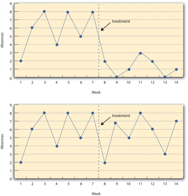
Imagine a study measuring student absences in a research methods course. The treatment in this study is the instructor publicly taking attendance each day, making students aware that their presence or absence is being recorded.

In the top panel of Figure 9.7.1, the treatment is effective. Before attendance tracking begins, absences remain consistently high week after week. Once the instructor starts taking attendance, there is an immediate and lasting drop in absences. This pattern suggests that the treatment successfully encouraged students to attend class more regularly.

In the bottom panel of Figure 9.7.1, the treatment is ineffective. Despite starting public attendance tracking, the number of absences remains roughly the same before and after the treatment. This indicates that the intervention had little to no impact on attendance.

This example highlights a key advantage of the interrupted time-series design compared to a simpler pretest-posttest design. If researchers had only measured absences once before and once after the treatment, for example, at Week 7 and Week 8, it might have appeared that any change between these two weeks was caused by the intervention. However, the multiple measurements before and after reveal whether changes in attendance are part of a consistent trend or just random fluctuations.

References

Cook, T. D., Campbell, D. T. (1979). Quasi-experimentation: Design & analysis issues for field settings. Houghton Mifflin.

Posternak, M. A., & Miller, I. (2001). Untreated short-term course of major depression: A meta-analysis of outcomes from studies using wait-list control groups. Journal of Affective Disorders, 66(2), 139–146. https://doi.org/10.1016/S0165-0327(00)00304-9