11.2. The t-Test
By Rajiv S. Jhangiani, I-Chant A. Chiang, Carrie Cuttler and Dana C. Leighton, adapted by Marc Chao and Muhamad Alif Bin Ibrahim
In psychology, many studies examine differences between two means, and the t-test is the most common tool for analysing such relationships. This section focuses on three types of t-tests, each suited to different research designs:
- One-Sample t-Test: Compares a sample mean to a known population mean.
- Dependent-Samples t-Test: Used when comparing two related groups, such as the same participants tested at different times.
- Independent-Samples t-Test: Compares the means of two independent groups, such as different sets of participants.
Even if you have taken a statistics course before, this section will help refresh your understanding of these essential tools.
One-Sample t-Test
The one-sample t-test is used to compare a sample mean (M) to a hypothetical population mean (μ0) that serves as a reference point. The test evaluates two competing hypotheses:
- Null Hypothesis (H0): The population mean (μ) equals the hypothetical mean (μ0).
- Alternative Hypothesis (H𝑎): The population mean (μ) is different from the hypothetical mean (μ0).
To decide between these hypotheses, the t-test calculates the probability (p-value) of obtaining a sample mean as extreme as the one observed if the null hypothesis were true. First, a statistic called t is calculated using this formula:
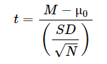
Here:
- M = Sample mean
- μ0 = Hypothetical population mean
- SD = Sample standard deviation
- N = Sample size
The Role of the t Distribution
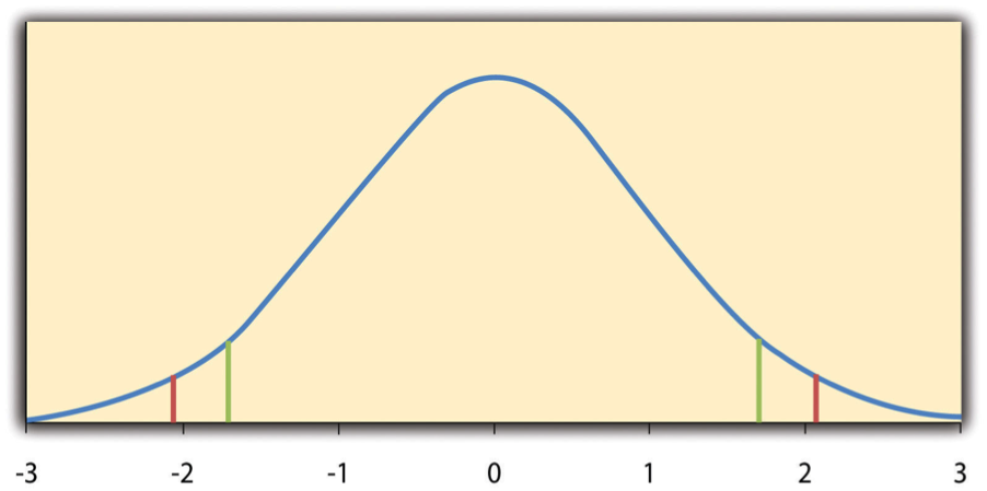
The t-statistic is useful because its behaviour under the null hypothesis is well understood as it follows a t distribution. This distribution is unimodal, symmetric, and centred at 0. Its shape depends on degrees of freedom (df), calculated as N − 1 for a one-sample t-test.
For example, with df = 24, the t distribution looks like Figure 11.2.1, where extreme t values occur in the tails. To calculate the p-value, the proportion of scores in the tails of this distribution that are as extreme as the observed t value is determined. For instance, a t value of 1.50 with df = 24 corresponds to a p-value of 0.14.
Decision Rule
Using statistical software, you can directly obtain the t value and p-value. Here’s how you interpret the results:
- If p ≤ 0.05, reject the null hypothesis and conclude that the population mean likely differs from the hypothetical mean.
- If p > 0.05, retain the null hypothesis, meaning there is insufficient evidence to conclude a difference.
When manually computing the t value, you can refer to a critical t-table (like Table 11.2.1). The table provides critical t values for different degrees of freedom (df) and significance levels (α = 0.05). For a two-tailed test, any t value beyond the critical values (e.g., ±2.064 for df = 24) leads to rejecting the null hypothesis.
| df | One-tailed | Two-tailed |
| Critical value | ||
| 3 | 2.353 | 3.182 |
| 4 | 2.132 | 2.776 |
| 5 | 2.015 | 2.571 |
| 6 | 1.943 | 2.447 |
| 7 | 1.895 | 2.365 |
| 8 | 1.860 | 2.306 |
| 9 | 1.833 | 2.262 |
| 10 | 1.812 | 2.228 |
| 11 | 1.796 | 2.201 |
| 12 | 1.782 | 2.179 |
| 13 | 1.771 | 2.160 |
| 14 | 1.761 | 2.145 |
| 15 | 1.753 | 2.131 |
| 16 | 1.746 | 2.120 |
| 17 | 1.740 | 2.110 |
| 18 | 1.734 | 2.101 |
| 19 | 1.729 | 2.093 |
| 20 | 1.725 | 2.086 |
| 21 | 1.721 | 2.080 |
| 22 | 1.717 | 2.074 |
| 23 | 1.714 | 2.069 |
| 24 | 1.711 | 2.064 |
| 25 | 1.708 | 2.060 |
| 30 | 1.697 | 2.042 |
| 35 | 1.690 | 2.030 |
| 40 | 1.684 | 2.021 |
| 45 | 1.679 | 2.014 |
| 50 | 1.676 | 2.009 |
| 60 | 1.671 | 2.000 |
| 70 | 1.667 | 1.994 |
| 80 | 1.664 | 1.990 |
| 90 | 1.662 | 1.987 |
| 100 | 1.660 | 1.984 |
One-Tailed vs. Two-Tailed Tests
Two-Tailed Test:
- Used when you suspect the sample mean might differ from the hypothetical mean, but do not know in which direction.
- Reject the null hypothesis if the t value falls in either tail of the distribution (e.g., below −2.064 or above +2.064 for df = 24).
One-Tailed Test:
- Applied when you expect a difference in a specific direction.
- You decide beforehand whether to test for a sample mean higher or lower than the hypothetical mean.
- For df = 24, one-tailed critical values are less extreme (±1.711). However, the disadvantage is that you lose the ability to detect differences in the opposite direction.
In both cases, the significance level (α = 0.05) is maintained. The one-tailed test gives more power to detect a directional difference but completely ignores the possibility of a difference in the opposite direction.
Example: One-Sample t-Test
A health psychologist is interested in evaluating how accurately university students estimate the calorie content of a chocolate chip cookie. The cookie contains 250 calories, which serves as the hypothetical population mean (μ0). The psychologist’s null hypothesis (H0) states that the population mean of students’ calorie estimates (μ) is equal to 250. Since he has no prior expectation about whether students overestimate or underestimate, he decides to conduct a two-tailed test to examine deviations in either direction.
To test the hypothesis, the psychologist gathers calorie estimates from a sample of 10 university students. Their individual estimates are as follows:
- 250, 280, 200, 150, 175, 200, 200, 220, 180, 250
From this data, the psychologist calculates the following sample statistics:
- Sample Mean (M): 212.00 calories
- Sample Standard Deviation (SD): 39.17 calories
- Sample Size (N): 10
The psychologist uses the one-sample t-test to determine if the sample mean significantly differs from the hypothetical population mean. The formula for the t-test is:
Where:
- M = Sample mean = 212.00
- μ0 = Hypothetical population mean = 250
- SD = Sample standard deviation = 39.17
- N = Sample size = 10
Substituting the values into the formula:
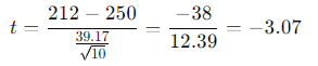
The computed t value is −3.07.
The psychologist enters the data into statistical software (e.g., SPSS or Excel). The software calculates the p value for this t-score with df = N − 1 = 10 − 1 = 9. The output shows a two-tailed p value of 0.013.
- Decision: Since p = 0.013 is less than the significance level α = 0.05, the psychologist rejects the null hypothesis.
- Conclusion: There is sufficient evidence to conclude that university students significantly underestimate the calorie content of a chocolate chip cookie.
If performing the test manually, the psychologist would consult a table of critical t values (e.g., Table 11.2.1). For a two-tailed test with df = 9 and α = 0.05, the critical value of t is:
tcritical = ±2.262
- The observed t value (t = −3.07) is more extreme than the critical value (−2.262), leading to the same conclusion: the null hypothesis is rejected.
The psychologist reports the results as follows:
- t(9) = −3.07, p = .01
Key formatting points in APA style include:
- The symbols t and p are italicised.
- The degrees of freedom (df) are placed in parentheses immediately after t.
- Both the t value and p value are rounded to two decimal places.
If the psychologist had a strong reason to believe that students would specifically underestimate the calories, a one-tailed test could be used. In this case:
- The critical value for df = 9 at α = 0.05 would be −1.833 (for the lower tail).
- Because t = −3.07 is more extreme than −1.833, the null hypothesis would still be rejected.
However, one-tailed tests have limitations. If the data showed an overestimation (a positive t value), the null hypothesis could not be rejected, as one-tailed tests only examine deviations in a pre-specified direction.
Dependent-Samples t-Test
The dependent-samples t-test, also called the paired-samples t-test, is used when comparing two means from the same group of participants. This test is typically applied in scenarios like pretest-posttest designs or within-subjects experiments, where each participant is tested under two conditions or at two different times.
Key Hypotheses
- Null hypothesis (H0): The population means for the two conditions or time points are the same (μ0 = 0).
- Alternative hypothesis (H𝑎): The population means for the two conditions or time points are different (μ0 ≠ 0).
If there is a clear expectation about the direction of the difference (e.g., an increase or decrease), a one-tailed test can be used instead of the more common two-tailed test.
How the Dependent-Samples t-Test Works
Think of the dependent-samples t-test as a variation of the one-sample t-test, with one additional step:
Calculate the difference scores:
- For each participant, compute the difference between their two scores (e.g., posttest score minus pretest score). These difference scores summarise the change for each individual.
Apply the One-Sample t-test:
- Once the difference scores are calculated, the test becomes a one-sample t-test conducted on the mean of the difference scores.
- The hypothetical population mean (μ0) for the difference scores is 0 because, under the null hypothesis, there is no average difference between the two conditions or time points.
Reframing the Hypotheses
- Under the null hypothesis, the mean difference score in the population is 0 (μ0 = 0).
- The alternative hypothesis states that the mean difference score in the population is not 0 (μ0 ≠ 0).
This approach allows the dependent-samples t-test to determine whether the observed differences between the two means are statistically significant, reflecting a real effect rather than random variation.
Example: Dependent-Samples t-Test
A health psychologist seeks to determine whether a specialised training program can enhance people’s ability to estimate the calorie content of junk food accurately. To test the program’s effectiveness, a pretest-posttest study is conducted with a sample of 10 participants. Each participant provides an estimate of the calories in a chocolate chip cookie before and after completing the training program. Since the psychologist expects the program to improve calorie estimates, a one-tailed test is used to analyse the data.
Pretest and Posttest Data Collection
The calorie estimates provided by the participants are recorded as follows:
- Pretest estimates: 230, 250, 280, 175, 150, 200, 180, 210, 220, 190
- Posttest estimates: 250, 260, 250, 200, 160, 200, 200, 180, 230, 240
The goal is to evaluate whether the posttest estimates, on average, are higher than the pretest estimates, indicating an improvement in accuracy due to the training.
To assess the change in estimates for each participant, the difference scores are calculated by subtracting the pretest estimates from the posttest estimates. A positive difference score indicates that a participant’s calorie estimate increased after the training, while a negative score indicates a decrease.
- Difference Score = Posttest Estimate − Pretest Estimate
The resulting difference scores are:
- Difference scores: 20, 10, −30, 25, 10, 0, 20, −30, 10, 50
The direction of subtraction (posttest minus pretest) does not matter as long as it is applied consistently for all participants.
From the difference scores, the following descriptive statistics are calculated:
- Mean of the difference scores (M): 8.50
- Standard deviation of the difference scores (SD): 27.27
- Sample size (N): 10
The null hypothesis (H0) states that the mean difference in calorie estimates after training is zero (μ0 = 0), implying no effect of the training program. The alternative hypothesis (HA) posits that the mean difference is greater than zero (μ > 0), consistent with an expected improvement.
The t-statistic is calculated using the following formula:
Where:
- M = Mean of the difference scores = 8.50
- μ0 = Hypothetical population mean = 0
- SD = Standard deviation of the difference scores = 27.27
- N = Sample size = 10
Substituting the values into the formula:
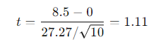
The calculated t value is 1.11.
The data can be entered into software such as SPSS, Excel, or an online t-test calculator. For df = N − 1 = 10 − 1 = 9, the one-tailed p value is 0.148.
- Decision: Since p = 0.148 is greater than the significance threshold (α = 0.05), the psychologist fails to reject the null hypothesis.
- Conclusion: There is insufficient evidence to conclude that the training program significantly improves calorie estimation accuracy.
If calculating by hand, the psychologist would refer to a critical t value table. For a one-tailed test with df = 9 and α = 0.05, the critical t value is 1.833.
- Comparison: The observed t value (t = 1.11) is less extreme than the critical value (t = 1.833).
- Decision: The psychologist fails to reject the null hypothesis, consistent with the software output.
The results suggest that the training program does not lead to a statistically significant improvement in calorie estimation. While the mean difference score (8.50) indicates a slight increase in posttest estimates, this difference is not large enough to rule out the possibility that it occurred by chance.
The Independent-Samples t-Test
The independent-samples t-test is used to compare the means (M1 and M2) of two separate groups. These groups may have been exposed to different conditions in a between-subjects experiment or represent naturally occurring categories in a cross-sectional study (e.g., women vs. men, extraverts vs. introverts).
Hypotheses
- Null hypothesis (H0): The population means are equal (μ1 = μ2).
- Alternative hypothesis (HA): The population means are not equal (μ1 ≠ μ2).
If there is strong evidence to expect a difference in a specific direction, a one-tailed test may be used instead of a two-tailed test.
Formula for the t-Statistic
The formula for the independent-samples t-test accounts for two sample means, their variances, and sample sizes. The t-statistic is calculated as:
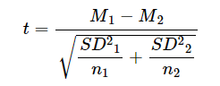
Where:
- M1 and M2: Sample means for the two groups.
- SD21 and SD22: Variances (squared standard deviations) for the two groups.
- n1 and n2: Sample sizes for the two groups.
Key Points
- Variances: The formula uses the squared standard deviations (variances) to reflect variability within each group. These variances are added together inside the square root symbol.
- Sample Sizes: The formula uses n1 and n2 to calculate the contribution of each group’s variance relative to its size.
- Degrees of Freedom: For the independent-samples t-test, the degrees of freedom are calculated as N − 2, where N is the total number of participants across both groups.
By combining the differences between the two group means, their variances, and sample sizes, the independent-samples t-test determines whether the observed difference is statistically significant.
Example: Independent-Samples t-Test
A health psychologist aims to investigate whether individuals who regularly consume junk food differ in their calorie estimates compared to those who rarely eat junk food. Since the psychologist does not have a clear hypothesis about the direction of the difference, a two-tailed test is chosen for the analysis.
The psychologist collects calorie estimation data from two independent groups:
- Junk food eaters (8 participants): 180, 220, 150, 85, 200, 170, 150, 190
- Mean (M1) = 168.12
- Standard deviation (SD1) = 42.66
- Non-junk food eaters (7 participants): 200, 240, 190, 175, 200, 300, 240
- Mean (M2) = 220.71
- Standard deviation (SD2) = 41.23
The goal is to determine if there is a statistically significant difference between the two groups’ calorie estimates.
Hypotheses
Null Hypothesis (H0): There is no difference between the population means of the two groups (μ1 = μ2).
Alternative Hypothesis (HA): There is a difference between the population means of the two groups (μ1 ≠ μ2).
The t-statistic formula for independent samples is:
Where:
- M1 and M2 are the sample means of the two groups.
- SD21 and SD22 are the variances (squared standard deviations) of the two groups.
- n1 and n2 are the sample sizes of the two groups.
Substituting the values into the formula:
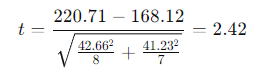
The calculated t-statistic is t = −2.42.
The psychologist inputs the data into statistical software such as SPSS, Excel, or an online t-test calculator. The software calculates a two-tailed p-value of 0.015 for t = −2.42 with df = 13 (degrees of freedom: N − 2 = 15 − 2).
- Decision: Since p = 0.015 is less than the significance threshold (α = 0.05), the psychologist rejects the null hypothesis.
- Conclusion: The results suggest that people who eat junk food regularly estimate fewer calories compared to those who rarely eat junk food.
To confirm the results, the psychologist refers to a t-distribution table. For a two-tailed test with df = 13 and α = 0.05, the critical t value is ±2.160.
- Comparison: The observed t value (−2.42) is more extreme than the critical value (−2.42 < −2.160).
- Decision: The null hypothesis is rejected.
The results can be reported as follows:
- t(13) = −2.42, p = .015
This format includes the degrees of freedom (df = 13), the t-statistic (t = −2.42), and the p-value (p = .015).
The analysis indicates a statistically significant difference between the calorie estimates of junk food eaters and non-junk food eaters. Specifically, junk food eaters provide lower calorie estimates compared to those who rarely eat junk food. This finding could suggest that regular junk food consumption might influence perceptions of calorie content, potentially contributing to dietary misjudgements.
Chapter Attribution
Content adapted, with editorial changes, from:
Research methods in psychology, (4th ed.), (2019) by R. S. Jhangiani et al., Kwantlen Polytechnic University, is used under a CC BY-NC-SA licence.
