By Rajiv S. Jhangiani, I-Chant A. Chiang, Carrie Cuttler and Dana C. Leighton, adapted by Marc Chao and Muhamad Alif Bin Ibrahim

In psychological research, it is common for studies to examine multiple levels of a single independent variable (e.g., placebo, new drug, old drug). However, it is equally common for experiments to include multiple independent variables within a single study. This approach allows researchers to explore more complex research questions. For example, Schnall and her colleagues (2008) studied whether physical disgust influences moral judgements by testing participants in either a clean or messy room and measuring their attention to bodily sensations (“private body consciousness”). Participants rated the moral acceptability of various behaviours and reported their current emotions. The study found that participants in the messy room felt more disgusted and made harsher moral judgements, but only if they had high private body consciousness. Hence, the researchers examined the effects of both disgust and private body consciousness in the same study.

The inclusion of multiple independent variables is further demonstrated by the following studies titles from professional journals:

• The Effects of Temporal Delay and Orientation on Haptic Object Recognition
• Opening Closed Minds: The Combined Effects of Intergroup Contact and Need for Closure on Prejudice
• Effects of Expectancies and Coping on Pain-Induced Intentions to Smoke
• The Effect of Age and Divided Attention on Spontaneous Recognition
• The Effects of Reduced Food Size and Package Size on the Consumption Behaviour of Restrained and Unrestrained Eaters

Including multiple independent variables, just like using multiple levels of a single independent variable, allows researchers to address more sophisticated research questions. For instance, rather than conducting two separate studies, one on how disgust influences moral judgement and another on how private body consciousness affects moral judgement, Schnall and her colleagues combined these questions into a single study.

Beyond efficiency, this approach enables researchers to investigate whether the effect of one independent variable depends on the level of another. This phenomenon is known as an interaction between independent variables. For example, Schnall and colleagues found an interaction between disgust and private body consciousness: the effect of disgust on moral judgement was influenced by whether participants had high or low levels of private body consciousness. Interactions, such as this one, often produce some of the most intriguing results in psychological research.

Factorial Designs

A factorial design is a common approach in experiments involving multiple independent variables, often referred to as factors. In this design, every level of one independent variable is combined with every level of the other(s), creating all possible combinations of conditions. Each combination represents a unique condition in the experiment.

Example: 2 × 2 Factorial Design

Consider an experiment investigating the effect of cell phone use (yes vs. no) and time of day (day vs. night) on driving ability. This design is shown in the factorial table in Figure 9.8.1, where:

• Columns represent cell phone use.
• Rows represent the time of day.
• Cells represent the four combinations:
  • Using a cell phone during the day.
  • Not using a cell phone during the day.
  • Using a cell phone at night.
  • Not using a cell phone at night.

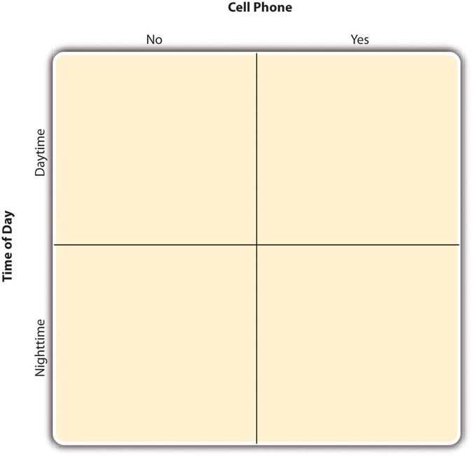
This setup is called a 2 × 2 factorial design (read as “two-by-two”) because it includes two independent variables, each with two levels.

Expanding Factorial Designs

If one variable includes a third level, for instance, differentiating between handheld cell phone use, hands-free cell phone use, and no cell phone use, the design becomes a 3 × 2 factorial design with six conditions. The total number of conditions is the product of the number of levels for each variable. For example:

• 2 × 2 design = 4 conditions.
• 3 × 2 design = 6 conditions.
• 4 × 5 design = 20 conditions.

The number of numbers in the factorial notation reflects the number of independent variables. For example:

• A 2 × 2 design has two independent variables, each with two levels.
• A 3 × 3 design also has two independent variables, but each has three levels.
• A 2 × 2 × 2 design has three independent variables, each with two levels.

Complex Designs and Practical Considerations

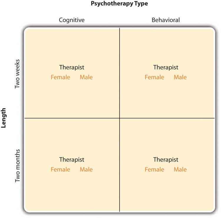
Factorial designs can theoretically include any number of independent variables with any number of levels. For example, a study might include:

• Type of psychotherapy (cognitive vs. behavioural),
• Length of therapy (2 weeks vs. 2 months),
• Therapist’s sex (female vs. male).

This would be a 2 × 2 × 2 factorial design, resulting in eight unique conditions. Figure 9.8.2 represents such a design.

However, adding more independent variables or levels can quickly make the design unmanageable:

1. Increased Conditions: Adding a fourth variable with three levels (e.g., therapist experience: low vs. medium vs. high) would create a 2 × 2 × 2 × 3 factorial design with 24 conditions.
2. Participant Requirements: More conditions require more participants to ensure adequate statistical power, making the design logistically and financially challenging.

For practical reasons, factorial designs typically involve no more than two or three independent variables, each with two or three levels. This simplifies the study while still allowing researchers to explore interactions between variables effectively. In this section, we focus on two-variable designs, though the principles discussed can be easily extended to more complex factorial designs.

Assigning Participants to Conditions

In a simple between-subjects design, each participant is tested in only one condition, whereas in a simple within-subjects design, each participant is tested in all conditions. In a factorial experiment, the decision to use a between-subjects or within-subjects approach must be made separately for each independent variable.

Between-Subjects Factorial Design

In a between-subjects factorial design, all independent variables are manipulated between subjects. For example, participants might be tested either while using a cell phone or not using a cell phone and either during the day or the night. Each participant would experience only one condition, ensuring they are tested in a single combination of the independent variables.

Advantages of this approach include its conceptual simplicity, the elimination of order or carryover effects, and the reduced time and effort required for participants. However, it often requires a larger number of participants to populate all conditions adequately.

Within-Subjects Factorial Design

In a within-subjects factorial design, all independent variables are manipulated within subjects. For example, participants might be tested both while using a cell phone and while not using a cell phone, and both during the day and the night. This means each participant would need to be tested in all four conditions.

The advantages of this design include greater efficiency for the researcher and better control over extraneous participant variables, such as individual differences. However, it may introduce order effects (where the sequence of conditions influences results) or carryover effects (where one condition affects performance in another). These issues can be mitigated through counterbalancing, where the order of conditions is varied systematically across participants.

Mixed Factorial Design

Since factorial designs involve multiple independent variables, it is also possible to use a mixed factorial design, where one independent variable is manipulated between subjects and another is manipulated within subjects.

For instance:

• Cell phone use could be a within-subjects factor, with participants tested both while using and not using a cell phone. Counterbalancing would ensure that the order of these two conditions varies across participants to prevent order effects.
• Time of day could be a between-subjects factor, with participants tested either during the day or at night. This approach might be chosen to minimise the burden on participants, as they would only need to attend a testing session once.

In this mixed design, each participant would experience two of the four possible conditions, combining the efficiency of within-subjects manipulation with the simplicity of between-subjects manipulation.

Regardless of whether a factorial design is between-subjects, within-subjects, or mixed, participants are typically assigned to conditions (or to the order of conditions) randomly. Random assignment ensures that differences between groups are distributed evenly, enhancing the validity of the study.

Non-Manipulated Independent Variables

In many factorial designs, one of the independent variables is non-manipulated. This means the researcher measures the variable but does not control or manipulate it. A study by Schnall and colleagues illustrates this distinction well. In their study, one independent variable, disgust, was manipulated by testing participants in either a clean or messy room. The other variable, private body consciousness, was a participant variable measured through a questionnaire.

Another example comes from a study by Halle Brown and colleagues, in which participants were asked to recall words they had previously seen (Brown et al., 1999). The manipulated independent variable was the type of word: some were health-related (e.g., tumour, coronary), while others were not health-related (e.g., election, geometry). The non-manipulated independent variable was participants’ level of hypochondriasis (excessive concern about ordinary bodily symptoms), which was measured. The results showed that participants with high hypochondriasis were better at recalling health-related words but not better at recalling non-health-related words compared to those with low hypochondriasis.

Key Points About Non-Manipulated Independent Variables

1. Typically Participant Variables: Non-manipulated independent variables are usually participant variables, such as private body consciousness, hypochondriasis, self-esteem, or gender. These are inherently between-subjects factors, as participants cannot belong to more than one level of these variables (e.g., being both high and low in hypochondriasis).
2. Experiments with Mixed Variables: Studies with both manipulated and non-manipulated variables are still generally considered experiments, as long as at least one independent variable is manipulated. The inclusion of non-manipulated variables does not diminish the experimental nature of the study.
3. Limits on Causal Conclusions: Causal conclusions can only be drawn about manipulated independent variables. For instance, Schnall and colleagues could conclude that disgust influenced the harshness of moral judgements because it was manipulated, and participants were randomly assigned to the clean or messy room. However, they could not conclude that private body consciousness caused harsher moral judgements because it was a non-manipulated variable. A third variable, such as neuroticism, might underlie both private body consciousness and moral strictness.

Thus, it is crucial to distinguish between manipulated and non-manipulated variables in a study to correctly interpret which variables can support causal inferences and which cannot.

Non-Experimental Studies With Factorial Designs

While factorial experiments often include manipulated independent variables or a combination of manipulated and non-manipulated variables, they can also consist solely of non-manipulated independent variables. In these cases, the design is no longer experimental but rather non-experimental in nature.

For instance, imagine a study where a researcher measures the moods and self-esteem of participants, categorising them as having either a positive or negative mood and either high or low self-esteem. The researcher also measures participants’ willingness to engage in unprotected sexual intercourse. This design can be conceptualised as a 2 × 2 factorial design, with mood (positive vs. negative) and self-esteem (high vs. low) as non-manipulated between-subjects factors. The dependent variable is participants’ willingness to engage in unprotected sex.

Since neither independent variable is manipulated in this example, the study is classified as non-experimental. This contrasts with an experimental study, such as the one by MacDonald and Martineau (2002), where participants’ moods were manipulated.

It is critical to exercise caution when interpreting results from non-experimental studies, particularly regarding causality. Non-experimental designs are vulnerable to issues like the directionality problem, where it is unclear whether one variable causes the other, and the third-variable problem, where an observed effect might be driven by another unmeasured variable. For example, if participants’ moods appear to influence their willingness to engage in unprotected sex, this relationship might actually be explained by another factor correlated with mood, such as personality traits or situational influences.

Graphing the Results of Factorial Experiments

In factorial experiments with two independent variables, the results are typically graphed with one independent variable represented on the x-axis and the other variable distinguished by different-coloured bars or lines. The y-axis always represents the dependent variable.

Figure 9.8.3 illustrates this process using two hypothetical factorial experiments.

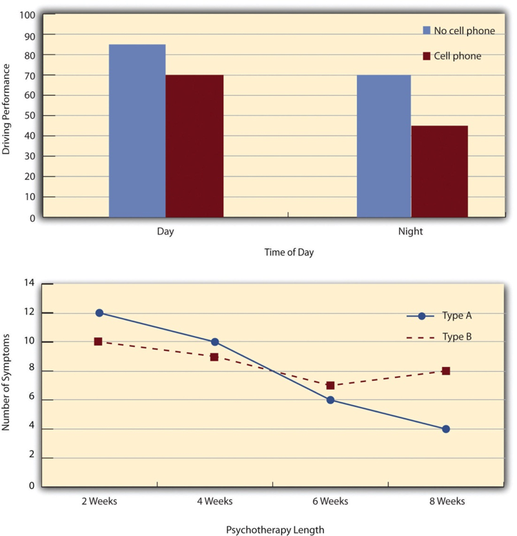
• Top Panel: This shows the results of a 2 × 2 factorial design, where time of day (day vs. night) is plotted along the x-axis, and cell phone use (no vs. yes) is depicted using bars of different colours. Alternatively, cell phone use could be shown on the x-axis, with time of day represented by the bar colours. The decision depends on which configuration makes the data easier to interpret.
• Bottom Panel: This represents the results of a 4 × 2 factorial design, where one variable, psychotherapy length, is quantitative and displayed on the x-axis. The other variable, psychotherapy type, is indicated by differently formatted lines. In this case, a line graph is used instead of a bar graph because the x-axis variable is quantitative with a limited number of distinct levels. Line graphs are also ideal for representing measurements over time, referred to as time series data.

Main Effects

In factorial designs, researchers are interested in three types of results: main effects, interaction effects, and simple effects. A main effect refers to the impact of one independent variable on the dependent variable, averaged across the levels of the other independent variable. Each independent variable in the study has its own main effect to consider.

The top panel of Figure 9.8.3 illustrates a main effect of cell phone use because, on average, driving performance was better when participants were not using cell phones compared to when they were. This is evident as the blue bars (no cell phone use) are higher, on average, than the red bars (cell phone use). Similarly, there is a main effect of time of day, as driving performance was better during the day than at night, regardless of cell phone use.

Main effects are independent of each other, meaning the presence or absence of a main effect for one independent variable does not indicate whether there is a main effect for another. For example, the bottom panel of Figure 9.8.3 shows a clear main effect of psychotherapy length: the longer the psychotherapy, the better the outcome, regardless of the other variable in the study. This independence allows researchers to evaluate each variable’s impact separately, providing a clearer understanding of the factors influencing the dependent variable.

Interactions

An interaction effect occurs when the effect of one independent variable depends on the level of another independent variable. While this may sound complex, the concept is quite intuitive. For example, imagine your friend invites you to a movie with another friend. Your response might be, “Well, it depends on which movie you’re seeing and who else is coming.” You are excited about the summer blockbuster but uninterested in the cheesy romantic comedy, which reflects a main effect of movie type. However, if your willingness to see the romantic comedy depends on whether your friend is bringing along someone you are interested in, there is an interaction. Similarly, drug interactions illustrate this concept. Viagra can be helpful for older men, and nitrates can effectively treat chest pain. However, taking both drugs together can be lethal, highlighting a critical interaction between the two medications.

Interactions are also prevalent in psychological research. For instance, the effect of receiving psychotherapy is stronger among people who are highly motivated to change compared to those who are not. This is an interaction because the effectiveness of psychotherapy depends on motivation levels. Similarly, Schnall and colleagues found an interaction in their study on moral judgements. The effect of a clean versus messy room on participants’ moral judgements depended on their level of private body consciousness. Participants high in private body consciousness made harsher judgements in a messy room, whereas participants low in private body consciousness were unaffected by the room’s condition.

In many studies, interactions are the primary focus of the research. For example, Brown and her colleagues hypothesised that individuals with hypochondriasis would recall negative health-related words more accurately than those without hypochondriasis but would recall non-health-related words at the same level as others. This hypothesis pointed to an interaction, and the results supported it.

Types of Interactions

The way one independent variable’s effect depends on the level of another independent variable can manifest in several ways. Two common types of interactions are spreading interactions and crossover interactions.

Spreading Interactions

In a spreading interaction, the effect of one independent variable is present at one level of the other independent variable but is weaker or absent at the other level. The top two panels of Figure 9.8.4 illustrate this:

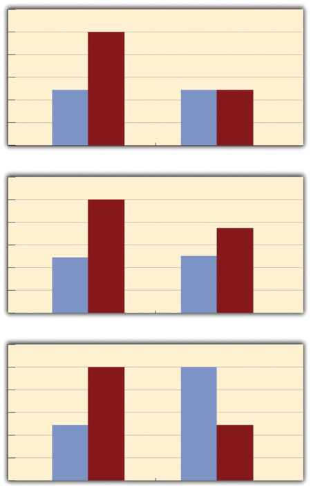
1. Effect at One Level Only: In the top panel, independent variable “B” has an effect at level 1 of independent variable “A” (indicated by the difference in the height of the blue and red bars on the left side of the graph). However, it has no effect at level 2 of independent variable “A” (the blue and red bars are the same height on the right side). This pattern is similar to Schnall and colleagues’ study, where disgust affected participants with high private body consciousness but had no effect on those with low private body consciousness.
2. Stronger Effect at One Level: In the middle panel, independent variable “B” has a stronger effect at level 1 of independent variable “A” than at level 2. This is indicated by a larger difference in the height of the blue and red bars on the left side compared to a smaller difference on the right side. An example of this is a hypothetical driving study where using a cell phone had a strong effect at night but a weaker effect during the day.

Crossover Interactions

A crossover interaction occurs when one independent variable affects both levels of the other independent variable, but the effects are in opposite directions. The bottom panel of Figure 9.8.4 demonstrates this: independent variable “B” produces opposite effects at levels 1 and 2 of independent variable “A.”

A real-world example of a crossover interaction comes from Kathy Gilliland’s study on the effect of caffeine on the verbal test scores of introverts and extraverts (Gilliland, 1980). Without caffeine, introverts perform better than extraverts. However, after consuming 4 mg of caffeine per kilogram of body weight, extraverts outperform introverts. This shows how the effect of caffeine depends on personality type.

Figure 9.8.5 provides examples of spreading and crossover interactions in line graphs where one independent variable is quantitative:

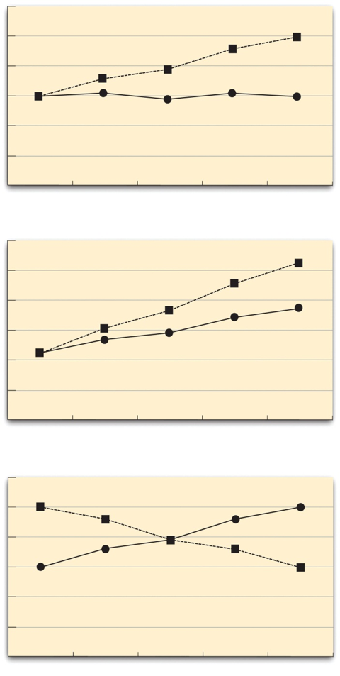
• Top Two Figures: These illustrate two types of spreading interactions. In each, the effect of one independent variable diminishes or disappears at certain levels of the other independent variable.
• Bottom Figure: This depicts a crossover interaction, where the two lines literally “cross over,” reflecting opposite effects of one independent variable at different levels of the other.

Simple Effects

When researchers find an interaction, it often reveals that the main effects may not tell the full story. Consider a crossover interaction where introverts outperform extraverts on a verbal memory test when they have not consumed caffeine, but extraverts outperform introverts when they have consumed caffeine. If researchers examine the main effect of caffeine consumption by averaging across introversion and extraversion, they might find no significant effect of caffeine overall, as the positive effect of caffeine for extraverts cancels out the negative effect for introverts. Similarly, examining the main effect of personality (introversion vs. extraversion) by averaging across caffeine conditions might show no overall effect, as the benefits of extraversion with caffeine balance out the drawbacks without it. However, the interaction suggests that the story is more complex because the effect of caffeine depends on personality.

To address this complexity, researchers use simple effects analyses, which break down the interaction to determine the effect of each independent variable at each level of the other independent variable. In this example, instead of averaging across personality, researchers would examine the effect of caffeine on introverts and then on extraverts. Similarly, they would analyse the effect of personality in the no-caffeine condition (where introverts performed better) and in the caffeine condition (where extraverts performed better). For a 2 × 2 design, this process results in two main effects and four simple effects analyses.

Examples of Simple Effects Analyses

Schnall and colleagues found a main effect of disgust on moral judgements, where participants in a messy room made harsher moral judgements overall. However, an interaction revealed that the effect of disgust depended on participants’ level of private body consciousness. Simple effects analyses showed that for individuals high in private body consciousness, disgust significantly influenced moral judgements. Conversely, for those low in private body consciousness, there was no effect of disgust on moral judgements. These analyses provided a clearer understanding of the interaction and revealed that the main effect of disgust was only accurate for part of the sample.

Similarly, Brown and colleagues studied the interaction between word type (health-related vs. non-health-related) and hypochondriasis (high vs. low) on word recall. Simple effects analyses examined the effect of hypochondriasis on health-related words and non-health-related words separately. Results showed that participants high in hypochondriasis recalled more health-related words than those low in hypochondriasis, but there was no difference in recall for non-health-related words. This analysis highlighted the specific nature of the interaction.

When to Use Simple Effects Analyses

Simple effects analyses are only necessary when an interaction is present. If no interaction exists, main effects analyses provide a complete and accurate picture. Unlike main effects analyses, which average across levels of the other independent variable, simple effects analyses examine the effect of one independent variable at each level of the other.

For example:

• A 2 × 2 design with four conditions involves 2 main effects and 4 simple effects.
• A 2 × 3 design with six conditions involves 2 main effects and 5 simple effects.
• A 3 × 3 design with nine conditions involves 2 main effects and 6 simple effects.

The number of main effects is determined by the number of independent variables, while the number of simple effects depends on the levels of the independent variables. Each simple effect examines one independent variable’s impact at a specific level of the other variable(s), providing detailed insights into how interactions shape the results.

References

Gilliland, K. (1980). The interactive effect of introversion-extraversion with caffeine induced arousal on verbal performance. Journal of Research in Personality, 14(4), 482–492. https://doi.org/10.1016/0092-6566(80)90006-9

MacDonald, T. K., & Martineau, A. M. (2002). Self-esteem, mood, and intentions to use condoms: When does low self-esteem lead to risky health behaviors? Journal of Experimental Social Psychology, 38(3), 299–306. https://doi.org/10.1006/jesp.2001.1505

Schnall, S., Haidt, J., Clore, G. L., & Jordan, A. H. (2008). Disgust as embodied moral judgment. Personality and Social Psychology Bulletin, 34(8), 1096-1109. https://doi.org/10.1177/0146167208317771

References

Brown, H. D., Kosslyn, S. M., Delamater, B., Fama, J., & Barsky, A. J. (1999). Perceptual and memory biases for health-related information in hypochondriacal individuals. Journal of Psychosomatic Research, 47(1), 67–78. https://doi.org/10.1016/S0022-3999(99)00011-2