10.3. Measures of Variability

By Rajiv S. Jhangiani, I-Chant A. Chiang, Carrie Cuttler and Dana C. Leighton, adapted by Marc Chao and Muhamad Alif Bin Ibrahim

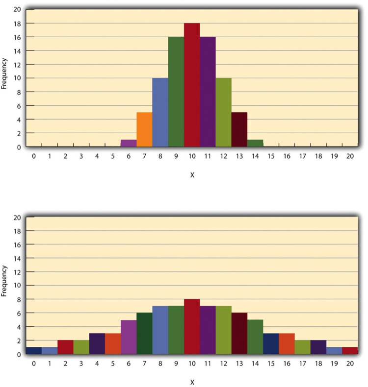
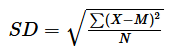
Variability tells us how spread out or clustered the scores are around the central point of a dataset. Even if two datasets have the same mean, median, and mode, they can still differ greatly in how much the scores vary. For example, Figure 10.3.1 shows two groups of students who both score an average of 10 on a test. In one group, most students score close to 10, while in the other group, scores are scattered widely between 2 and 18. These differences in variability reveal important information about the data.

The Range

The range is the simplest measure of variability. It is calculated by subtracting the lowest score from the highest score:

• Range = Highest Score − Lowest Score

For example, if the highest self-esteem score is 24 and the lowest is 15, the range would be:

• 24 − 15 = 9

While the range is easy to calculate and understand, it has a significant limitation: it is heavily influenced by outliers (extremely high or low scores). For instance, if most students score between 90 and 100 on an exam but one student scores 20, the range increases dramatically, making the data seem more variable than it actually is.

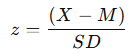
The Standard Deviation

The standard deviation is the most commonly used measure of variability because it gives a more precise picture of how scores are spread around the mean. It measures the average distance between each score and the mean.

For example:

• In a dataset with low variability, most scores will be close to the mean, resulting in a small standard deviation.
• In a dataset with high variability, scores will be spread out far from the mean, leading to a large standard deviation.

In Figure 10.3.1:

• The top distribution has a standard deviation of 1.69, showing that most scores are close to the mean.
• The bottom distribution has a standard deviation of 4.30, indicating that the scores are more widely spread out.

Calculating the standard deviation involves several steps:

1. Find the difference between each score and the mean.
2. Square each difference.
3. Calculate the mean of these squared differences (this is called the variance).
4. Take the square root of the variance.

Mathematically, it looks like this:

• SD: Standard deviation
• Σ (Sigma): Sum of all values
• X: Individual score
• M: Mean of the scores
• N: Total number of scores

This formula might look complicated, but it simply ensures that every score’s distance from the mean is considered, and squaring the differences eliminates negative values.

Variance

In the process of calculating the standard deviation, there is an intermediate step called the variance (symbolized as SD²). Variance is the mean of the squared differences from the mean. While it is less intuitive than the standard deviation, variance is important for more advanced statistical techniques, especially in inferential statistics.

For practical purposes in descriptive statistics:

Standard deviation is the preferred measure because it is in the same units as the original data (e.g., if data is in seconds, the standard deviation is also in seconds).
Variance, on the other hand, is expressed in squared units, which makes it harder to interpret directly.

Percentile Ranks and z-Scores

When analysing data, it is often helpful to know where an individual score falls within a larger dataset. Two common ways to describe a score’s position are percentile ranks and z-scores.

Percentile Ranks

A percentile rank shows what percentage of scores in a dataset are lower than a specific score.

For example:

• In a dataset of 40 self-esteem scores (as shown in Table 10.1.1), suppose five students scored 23.
• By counting how many students scored lower than 23, we find that 32 students (80%) had lower scores.
• Therefore, a score of 23 corresponds to the 80th percentile, meaning those students scored higher than 80% of their peers.

Percentile ranks are especially common in standardised testing. For instance:

• If your percentile rank on a verbal ability test is 40, it means you scored higher than 40% of the people who took the test.

Percentiles provide a quick and easy way to compare individual performance against a larger group.

z-Scores

While percentile ranks tell us about a score’s relative position, z-scores offer a precise measurement of how far a score is from the mean, expressed in standard deviation units.

The formula for calculating a z-score is:

• X: The individual score
• M: The mean of the dataset
• SD: The standard deviation

For example:

In an IQ score dataset where:

• Mean (M) = 100
• Standard deviation (SD) = 15

An individual with an IQ score of 110 would calculate their z-score as:

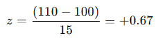
This means the score is 0.67 standard deviations above the mean.

Similarly, an IQ score of 85 would calculate as:

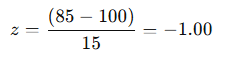
This means the score is 1 standard deviation below the mean.

z-scores are valuable because they:

• Show a Score’s Position in a Dataset: They clearly indicate how far a score is from the average in standardised units.
• Identify Outliers: Scores with z-scores below −3.00 or above +3.00 are often considered outliers because they fall more than three standard deviations from the mean.
• Enable Comparisons Across Different Datasets: Because z-scores standardise data, they allow comparisons between different datasets with different means and standard deviations.
• Support Advanced Statistical Calculations: z-scores are often used as building blocks for other statistical analyses, which we will explore later.