11.1. Null Hypothesis Testing
By Rajiv S. Jhangiani, I-Chant A. Chiang, Carrie Cuttler and Dana C. Leighton, adapted by Marc Chao and Muhamad Alif Bin Ibrahim
In psychological research, scientists often measure one or more variables in a sample and then calculate descriptive statistics, such as means or correlation coefficients, to summarise the data. These statistics provide useful insights about the sample, but the ultimate goal of most research is to make conclusions about the larger population from which the sample was drawn. In statistics, these population values are called parameters.
For example, imagine a researcher measures the number of depressive symptoms in 50 adults diagnosed with clinical depression and calculates the average number of symptoms in that sample. The researcher is not just interested in the average for that specific group but wants to make an inference about the average number of depressive symptoms across all adults with clinical depression.
However, sample statistics are imperfect estimates of population parameters because of random variability, a phenomenon known as sampling error. Even if samples are selected randomly from the same population, the statistics can vary. For instance, in one sample, the average number of depressive symptoms might be 8.73, while in another it might be 6.45, and in a third, it could be 9.44. Similarly, the correlation between two variables might show values like +0.24, -0.04, or +0.15 across different samples. This variability is normal and expected, and it does not mean anyone made a mistake, it is simply the result of random chance.
This variability creates a challenge: when researchers observe a statistical relationship in a sample, it is not always clear whether the relationship truly exists in the population or if it is just a result of sampling error.
For example, a small difference between two group means in a sample might suggest a real difference in the population. However, it could also mean that no real difference exists, and the observed difference is merely due to random variation. Similarly, a correlation value of -0.29 in a sample might indicate a negative relationship in the population, or it might just be noise caused by sampling error.
In essence, every statistical relationship in a sample has two possible explanations:
- The relationship exists in the population, and the sample reflects this real relationship.
- There is no real relationship in the population, and the sample result is simply due to sampling error.
The purpose of null hypothesis testing is to help researchers distinguish between these two possibilities and make informed conclusions about whether the patterns they see in their data are likely to reflect real relationships in the population.
The Logic of Null Hypothesis Testing
Null hypothesis testing (often called null hypothesis significance testing or NHST) is a statistical method used to determine whether a relationship observed in a sample reflects a real relationship in the population or if it simply occurred by chance.
At the core of NHST are two competing explanations: the null hypothesis (H₀) and the alternative hypothesis (H₁). The null hypothesis suggests that there is no real relationship in the population and that any observed relationship in the sample is due to random chance or sampling error. In simpler terms, it assumes that the sample result is just a coincidence. The alternative hypothesis, on the other hand, proposes that there is a real relationship in the population and that the sample result reflects this genuine relationship.
Every statistical result in a sample can be interpreted in one of these two ways: either it happened by chance, or it represents a real relationship in the population. Researchers need a systematic way to decide between these two interpretations, and NHST provides that framework.
The process follows a clear logic. First, researchers assume the null hypothesis is true, meaning they start from the assumption that there is no relationship in the population. Then they calculate how likely the sample result (or one even more extreme) would be if the null hypothesis were true. If the result is extremely unlikely under the null hypothesis, researchers reject the null hypothesis in favour of the alternative hypothesis. If the result is not extremely unlikely, they fail to reject the null hypothesis and conclude that there is not enough evidence to claim a real relationship exists.
To illustrate, consider the study by Mehl and colleagues, who investigated differences in talkativeness between men and women. They asked, “If there were no real difference in talkativeness in the population, how likely would it be to observe a difference of d = 0.06 in our sample?” Their analysis showed that such a small difference was fairly likely under the null hypothesis. As a result, they failed to reject the null hypothesis and concluded there was no evidence of a meaningful difference in the population.
In contrast, Kanner and colleagues examined the correlation between daily hassles and symptoms. They asked, “If there were no real correlation in the population, how likely would it be to observe a strong correlation of +0.60 in our sample?” Their analysis indicated that such a strong correlation would be very unlikely under the null hypothesis. Therefore, they rejected the null hypothesis and concluded that there is a positive correlation between these variables in the population.
A key step in NHST is determining the p-value, which represents the probability of obtaining a sample result (or one even more extreme) if the null hypothesis were true. A low p-value indicates that the result is unlikely under the null hypothesis, leading researchers to reject the null hypothesis. A high p-value, on the other hand, suggests that the result could reasonably occur by chance, so researchers fail to reject the null hypothesis.
But how low must a p-value be to reject the null hypothesis? Researchers typically use a threshold called alpha (α), which is almost always set at 0.05. If the p-value is 0.05 or lower, it means there is less than a 5% chance of obtaining such an extreme result if the null hypothesis were true. In this case, the result is considered statistically significant, and the null hypothesis is rejected. If the p-value is greater than 0.05, the null hypothesis is not rejected, but this does not mean it is accepted as true, only that there is not enough evidence to reject it.
To avoid confusion, researchers avoid saying they “accept” the null hypothesis. Instead, they use the phrase “fail to reject the null hypothesis”, emphasising that the evidence simply was not strong enough to support rejecting it.
Understanding these principles is crucial for interpreting statistical results accurately and avoiding common misunderstandings about what a p-value really represents.
The Misunderstood p-Value
The p-value is one of the most frequently misunderstood concepts in psychological research, even among experienced researchers. Misinterpretations of the p-value are so common that they sometimes appear in statistics textbooks as well.
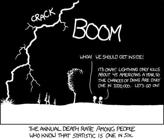
A widespread mistake is thinking that the p-value represents the probability that the null hypothesis is true or the likelihood that the sample result happened purely by chance (Figure 11.1.1). For example, someone might incorrectly conclude that a p-value of 0.02 means there is only a 2% chance that the result was due to random chance and a 98% chance that the observed relationship is real. This interpretation is wrong.
In reality, the p-value indicates the probability of obtaining a result as extreme as the one observed (or more extreme) if the null hypothesis were true. A p-value of 0.02 means that if there were truly no relationship in the population (if the null hypothesis were correct), a sample result this extreme would occur only 2% of the time due to random chance.
To avoid this common misunderstanding, it is essential to remember that the p-value does not tell us the probability that the null hypothesis is true or false. Instead, it tells us how likely it is to observe the sample result (or something even more extreme) under the assumption that the null hypothesis is correct.

Role of Sample Size and Relationship Strength
Null hypothesis testing seeks to answer this question: “If the null hypothesis were true, what is the probability of observing a sample result as extreme as this one?” This probability is the p-value, and it depends on two key factors: the strength of the relationship and the sample size. Specifically, stronger relationships and larger samples make it less likely that the observed result would occur if the null hypothesis were true, leading to a lower p-value.
To clarify, imagine two scenarios:
- Large sample, strong relationship: Suppose you compare a sample of 500 women and 500 men on a psychological characteristic, and Cohen’s d is a strong 0.50. If there were truly no sex difference in the population, such a strong result from such a large sample would be very unlikely. The null hypothesis would likely be rejected.
- Small sample, weak relationship: Now imagine a similar study comparing three women and three men, but Cohen’s d is a weak 0.10. If there were no sex difference in the population, this weak result from such a small sample would be entirely plausible. The null hypothesis would likely be retained.
This explains why strong results in large samples are more likely to lead to rejecting the null hypothesis, while weak results in small samples are not.
However, the relationship between these two factors is not always so straightforward. A weak result can still be statistically significant if the sample is very large, and a strong relationship can be significant even with a small sample. This trade-off between relationship strength and sample size is summarised in Table 11.1.1, which provides a rough guideline for determining statistical significance.
| Relationship strength | |||
| Sample Size | Weak | Medium | Strong |
| Small (N = 20) | No | No | d = Mayber = Yes |
| Medium (N = 50) | No | Yes | Yes |
| Large (N = 100) | d = Yesr = No | Yes | Yes |
| Extra large (N = 500) | Yes | Yes | Yes |
From Table 11.1.1:
- Weak relationships: These are never statistically significant in small or medium samples but can be significant in very large samples.
- Strong relationships: These are always statistically significant with medium or larger samples and sometimes even with small samples, depending on specific factors.
This understanding is invaluable for developing intuitive judgement about statistical significance. For instance, if you observe a strong relationship with a medium sample, you should expect to reject the null hypothesis. If the formal test suggests otherwise, it signals a need to review your computations or interpretations.
Statistical Significance vs. Practical Significance
Statistical significance and practical significance are two different but equally important concepts in interpreting research results. A result can be statistically significant without being practically meaningful. This distinction is crucial because statistical significance only tells us that an observed effect is unlikely to have occurred by random chance, not whether the effect is strong or useful in a real-world context (Figure 11.1.2).
For example, Janet Shibley Hyde highlighted findings on sex differences in areas like mathematical problem-solving and leadership ability. While these differences are often statistically significant, they are usually so small that they have little practical relevance. Despite their statistical significance, these findings should not influence major decisions, such as which college courses to pursue or whom to vote for.
This distinction becomes even more important in fields like clinical psychology. A study might find that a new treatment for social phobia produces a statistically significant improvement in symptoms. However, if the improvement is very small, it might not justify the costs, time, and effort required to implement the treatment, especially if existing treatments deliver similar or better results.
In such cases, researchers refer to this concept as clinical significance, which focuses on whether the effect is meaningful or useful in a practical setting. Even if a study meets the statistical threshold for significance, it might lack real-world impact if the effect size is minimal or the costs outweigh the benefits.
Chapter Attribution
Content adapted, with editorial changes, from:
Research methods in psychology, (4th ed.), (2019) by R. S. Jhangiani et al., Kwantlen Polytechnic University, is used under a CC BY-NC-SA licence.
