11.3. The Analysis of Variance
By Rajiv S. Jhangiani, I-Chant A. Chiang, Carrie Cuttler and Dana C. Leighton, adapted by Marc Chao and Muhamad Alif Bin Ibrahim
While t-tests are ideal for comparing two means, such as between a sample mean and a population mean, or between the means of two groups or conditions, they are not suitable when more than two groups or conditions need to be compared. For these cases, the analysis of variance (ANOVA) is the most common statistical method.
This section focuses primarily on the one-way ANOVA, which is used in between-subjects designs with a single independent variable. Additionally, it provides a brief overview of other types of ANOVA, such as those used in within-subjects designs and factorial designs.
One-Way ANOVA
The one-way ANOVA is a statistical test used to compare the means of more than two groups (e.g., M1, M2…MG) in a between-subjects design. It is particularly useful when the research involves multiple conditions or groups.
The null hypothesis for a one-way ANOVA is that all group means are equal in the population (μ1 = μ2 = ⋯ = μ𝐺). The alternative hypothesis asserts that not all means are equal.
The F Statistic in ANOVA
The test statistic for ANOVA is called F, which is calculated as the ratio of two estimates of population variance derived from the sample data:
- Mean Squares Between Groups (MSB): This measures variability between the group means.
- Mean Squares Within Groups (MSW): This measures variability within each group.
The formula for the F statistic is:
F = MSB / MSW
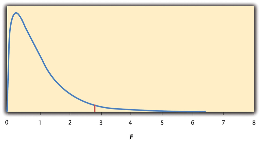
This statistic is useful because we know how it behaves under the null hypothesis. As shown in Figure 11.3.1, the F-distribution is unimodal and positively skewed, with most values clustering around 1 when the null hypothesis is true. The shape of the distribution depends on two types of degrees of freedom:
- Between-groups degrees of freedom: dfB = G − 1, where G is the number of groups.
- Within-groups degrees of freedom: dfW = N − G, where N is the total sample size.
Interpreting F and the p-Value
By knowing the distribution of F under the null hypothesis, we can calculate the p-value. Statistical software like SPSS or Excel can compute both the F statistic and the p-value.
- If p ≤ 0.05, reject the null hypothesis and conclude that there are differences among the group means.
- If p > 0.05, retain the null hypothesis, as there is not enough evidence to conclude differences exist.
Using Critical Values to Interpret F
In cases where F is calculated manually, a table of critical values (like Table 11.3.1) can be used. For example:
- If the computed F ratio exceeds the critical value for the given degrees of freedom (dfB and dfW), the null hypothesis is rejected.
- If the computed F ratio is less than the critical value, the null hypothesis is retained.
- Critical values vary based on the degrees of freedom and the significance level (α = 0.05).
| dfB | |||
| dfW | 2 | 3 | 4 |
| 8 | 4.459 | 4.066 | 3.838 |
| 9 | 4.256 | 3.863 | 3.633 |
| 10 | 4.103 | 3.708 | 3.478 |
| 11 | 3.982 | 3.587 | 3.357 |
| 12 | 3.885 | 3.490 | 3.259 |
| 13 | 3.806 | 3.411 | 3.179 |
| 14 | 3.739 | 3.344 | 3.112 |
| 15 | 3.682 | 3.287 | 3.056 |
| 16 | 3.634 | 3.239 | 3.007 |
| 17 | 3.592 | 3.197 | 2.965 |
| 18 | 3.555 | 3.160 | 2.928 |
| 19 | 3.522 | 3.127 | 2.895 |
| 20 | 3.493 | 3.098 | 2.866 |
| 21 | 3.467 | 3.072 | 2.840 |
| 22 | 3.443 | 3.049 | 2.817 |
| 23 | 3.422 | 3.028 | 2.796 |
| 24 | 3.403 | 3.009 | 2.776 |
| 25 | 3.385 | 2.991 | 2.759 |
| 30 | 3.316 | 2.922 | 2.690 |
| 35 | 3.267 | 2.874 | 2.641 |
| 40 | 3.232 | 2.839 | 2.606 |
| 45 | 3.204 | 2.812 | 2.579 |
| 50 | 3.183 | 2.790 | 2.557 |
| 55 | 3.165 | 2.773 | 2.540 |
| 60 | 3.150 | 2.758 | 2.525 |
| 65 | 3.138 | 2.746 | 2.513 |
| 70 | 3.128 | 2.736 | 2.503 |
| 75 | 3.119 | 2.727 | 2.494 |
| 80 | 3.111 | 2.719 | 2.486 |
| 85 | 3.104 | 2.712 | 2.479 |
| 90 | 3.098 | 2.706 | 2.473 |
| 95 | 3.092 | 2.700 | 2.467 |
| 100 | 3.087 | 2.696 | 2.463 |
Example: One-Way ANOVA
A health psychologist is investigating whether different groups estimate the calorie content of a chocolate chip cookie differently. The three groups in the study are psychology majors, nutrition majors, and professional dietitians. The psychologist collects calorie estimation data from participants in each group and compares the group means using a one-way ANOVA. This statistical test is designed to determine if there are significant differences among the group means in the population.
The calorie estimates from each group are as follows:
- Psychology majors (8 participants): 200, 180, 220, 160, 150, 200, 190, 200
- Mean (M1) = 187.50
- Standard Deviation (SD1) = 23.14
- Nutrition majors (9 participants): 190, 220, 200, 230, 160, 150, 200, 210, 195
- Mean (M2) = 195.00
- Standard Deviation (SD2) = 27.77
- Dieticians (8 participants): 220, 250, 240, 275, 250, 230, 200, 240
- Mean (M3) = 238.13
- Standard Deviation (SD3) = 22.35
From the descriptive statistics, it appears that dieticians provide significantly higher calorie estimates than both psychology and nutrition majors.
Hypotheses
- Null Hypothesis (H0): The mean calorie estimates for the three groups are equal in the population (μ1 = μ2 = μ3).
- Alternative Hypothesis (HA): At least one of the group means is significantly different from the others.
The psychologist decides to run a one-way ANOVA to statistically test whether the group means are significantly different in the population. The psychologist uses statistical software (e.g., SPSS, Excel, or another tool) to conduct the one-way ANOVA. The software calculates the F ratio and the p-value to determine whether the differences among the group means are statistically significant.
The results of the ANOVA are summarised in the following table (Table 11.3.2):
| Source of variation | SS | df | MS | F | p-value | Fcritical |
| Between groups | 11,943.75 | 2 | 5,971.875 | 9.916234 | 0.000928 | 3.4668 |
| Within groups | 12,646.88 | 21 | 602.2321 | |||
| Total | 24,590.63 | 23 |
Key results from the table:
- MSB (mean squares between groups): 5,971.88
- MSW (mean squares within groups): 602.23
- F (F ratio): 9.92
- p-value: 0.0009
Interpretation of Results
- Decision rule: The critical value of F (Fcritical) at α = 0.05, with 2 and 21 degrees of freedom, is 3.467. The computed F ratio (9.92) exceeds this critical value, indicating that the result is statistically significant.
- p-value: The p-value (0.0009) is much smaller than 0.05, providing strong evidence to reject the null hypothesis.
- Conclusion: The psychologist concludes that the mean calorie estimates for the three groups are not equal in the population. This suggests significant differences in how the three groups estimate calorie content.
The results provide strong evidence that dieticians estimate calories differently from the other two groups. However, the ANOVA does not specify which group means are different from each other. To identify the specific group differences, post hoc comparisons (e.g., Tukey’s HSD test) would need to be conducted.
The results can be reported as follows:
- F(2, 21) = 9.92, p = 0.0009
This format indicates:
- Degrees of freedom (dfB = 2, dfW = 21)
- F-statistic (F = 9.92)
- p-value (p = 0.0009)
The sum of squares (SS) values for “Between Groups” and “Within Groups” are intermediate calculations used to find the MSB and MSW values but are not typically reported in the final results.
If the F ratio had been computed manually, the psychologist could use a table of critical values (like Table 11.3.1) to confirm the statistical significance.
Post Hoc Comparisons: Follow-Up Tests After ANOVA
When the null hypothesis is rejected in a one-way ANOVA, we conclude that the group means are not all equal in the population. However, this result does not clarify the specific nature of the differences. For instance, in a study with three groups:
- All three means might differ significantly from one another. For example, the mean calorie estimates for psychology majors, nutrition majors, and dieticians could all be distinct.
- Only one mean might differ significantly. For example, dieticians’ calorie estimates might differ significantly from those of psychology and nutrition majors, while the psychology and nutrition majors’ means remain similar.
Because ANOVA does not specify which groups differ, significant results are typically followed by post hoc comparisons to identify specific group differences.
Why Not Just Use Multiple t-Tests?
A straightforward approach might be to run a series of independent-samples t-tests, comparing each group’s mean to every other group. However, this method has a critical flaw: increased risk of type I errors. Each t-test has a 5% chance of incorrectly rejecting the null hypothesis when it is true. Conducting multiple t-tests increases the cumulative probability of making at least one error. For example, with three groups, conducting three t-tests raises the likelihood of a mistake beyond the acceptable 5% level.
To control for this inflated error risk, researchers use modified t-test procedures designed to keep the overall error rate within acceptable limits (close to 5%). These methods include:
- Bonferroni Procedure: Adjusts the significance threshold for each test based on the number of comparisons.
- Fisher’s Least Significant Difference (LSD) Test: Performs comparisons but with adjustments to maintain accuracy.
- Tukey’s Honestly Significant Difference (HSD) Test: Specifically designed for pairwise comparisons to control error rates.
While the technical details of these methods are beyond the scope of this explanation, their purpose is straightforward: to minimise the chance of mistakenly rejecting a true null hypothesis while identifying meaningful group differences.
Repeated-Measures ANOVA
The one-way ANOVA is designed for between-subjects designs, where the means being compared come from separate groups of participants. However, it is not suitable for within-subjects designs, where the same participants are tested under different conditions or at different times. In these cases, a repeated-measures ANOVA is used instead.
The fundamental principles of repeated-measures ANOVA are similar to those of the one-way ANOVA. The primary distinction lies in how the analysis accounts for variability within the data:
Handling Individual Differences
Measuring the dependent variable multiple times for each participant allows the analysis to account for stable individual differences. These are characteristics that consistently vary among participants but remain unchanged across conditions. For example:
- In a reaction-time study, some participants might be naturally faster or slower due to stable factors like their nervous system or muscle response.
- In a between-subjects design, these differences add to the variability within groups, increasing the mean squares within groups (MSW). A higher MSW results in a lower F value, making it harder to detect significant differences.
- In a repeated-measures design, these stable individual differences are measured and subtracted from MSW, reducing its value.
Increased Sensitivity
By reducing the value of MSW, repeated-measures ANOVA produces a higher F value, making the test more sensitive to detecting actual differences between conditions.
This approach leverages the fact that participants serve as their own control, allowing the analysis to isolate and remove irrelevant variability caused by stable individual differences. As a result, repeated-measures ANOVA offers a more precise and powerful way to detect meaningful effects in within-subjects designs.
Factorial ANOVA
When a study includes more than one independent variable, the appropriate statistical approach is the factorial ANOVA. This method builds on the principles of the one-way and repeated-measures ANOVAs but is designed to handle the complexities of factorial designs.
Multiple Effects Analysis
Factorial ANOVA examines not only the impact of each independent variable (main effects) but also how these variables interact (interaction effects). For each:
- It calculates an F ratio to measure the variability explained by the effect.
- It provides a p value to indicate whether the effect is statistically significant.
Main Effects
These represent the individual influence of each independent variable on the dependent variable. For example:
- In a calorie estimation study, one main effect might measure whether a participant’s major (psychology vs. nutrition) influences calorie estimates.
- Another main effect might examine whether the type of food (cookie vs. hamburger) affects the estimates.
Interaction Effects
The interaction effect explores whether the influence of one independent variable depends on the level of the other. For instance:
- Does the participant’s major (psychology vs. nutrition) affect calorie estimates differently depending on the type of food (cookie vs. hamburger)?
Customising for Study Design
The factorial ANOVA is adaptable and must be tailored based on the study design:
- Between-subjects design: Participants are assigned to separate groups based on the levels of the independent variables.
- Within-subjects design: The same participants experience all levels of the independent variables.
- Mixed design: Combines between-subjects and within-subjects elements.
Imagine a health psychologist investigates calorie estimation using two independent variables: participant major (psychology vs. nutrition) and food type (cookie vs. hamburger). A factorial ANOVA would calculate:
- An F ratio and p value for the main effect of major.
- An F ratio and p value for the main effect of food type.
- An F ratio and p value for the interaction between major and food type.
This analysis provides a detailed understanding of how the independent variables individually and collectively influence calorie estimates, making the factorial ANOVA a powerful tool for complex research designs.
Chapter Attribution
Content adapted, with editorial changes, from:
Research methods in psychology, (4th ed.), (2019) by R. S. Jhangiani et al., Kwantlen Polytechnic University, is used under a CC BY-NC-SA licence.
