3.6 Quantitative Data Analysis
Remember that quantitative research explains phenomena by collecting numerical data that are analysed using statistics.1 Statistics is a scientific method of collecting, processing, analysing, presenting and interpreting data in numerical form.44 This section discusses how quantitative data is analysed and the choice of test statistics based on the variables (data). First, it is important to understand the different types of variables before delving into the statistical tests.
Types of variables
A variable is an item (data) that can be quantified or measured. There are two main types of variables – numerical variables and categorical variables.45 Numerical variables describe a measurable quantity and are subdivided into two groups – discrete and continuous data. Discrete variables are finite and are based on a set of whole values or numbers such as 0, 1, 2, 3,… (integer). These data cannot be broken into fractions or decimals.45 Examples of discrete variables include the number of students in a class and the total number of states in Australia. Continuous variables can assume any value between a certain set of real numbers e.g. height and serum glucose levels. In other words, these are variables that are in between points (101.01 to 101.99 is between 101 and 102) and can be broken down into different parts, fractions and decimals.45
On the other hand, categorical variables are qualitative and describe characteristics or properties of the data. This type of data may be represented by a name, symbol or number code.46 There are two types- nominal and ordinal variables. Nominal data are variables having two or more categories without any intrinsic order to the categories.46 For example, the colour of eyes (blue, brown, and black) and gender (male, female) have no specific order and are nominal categorical variables. Ordinal variables are similar to nominal variables with regard to describing characteristics or properties, but these variables have a clear, logical order or rank in the data.46 The level of education (primary, secondary and tertiary) is an example of ordinal data.
Now that you understand the different types of variables, identify the variables in the scenario in the Padlet below.
Statistics
Statistics can be broadly classified into descriptive and inferential statistics. Descriptive statistics explain how different variables in a sample or population relate to one another.60 Inferential statistics draw conclusions or inferences about a whole population from a random sample of data.45
Descriptive statistics
This is a summary description of measurements (variables) from a given data set, e.g., a group of study participants. It provides a meaningful interpretation of the data. It has two main measures – central tendency and dispersion measures.45
The measures of central tendency describe the centre of data and provide a summary of data in the form of mean, median and mode. Mean is the average distribution, the median is the middle value (skewed distribution), and mode is the most frequently occurring variable.4

The measures of dispersion describe the spread of data, including range, variance, and standard deviation.45 The range defines the spread of the data, and it is described by the maximum and minimum values of the data. Variance is the average degree to which each point differs from the mean. The standard deviation is the square root of variance.45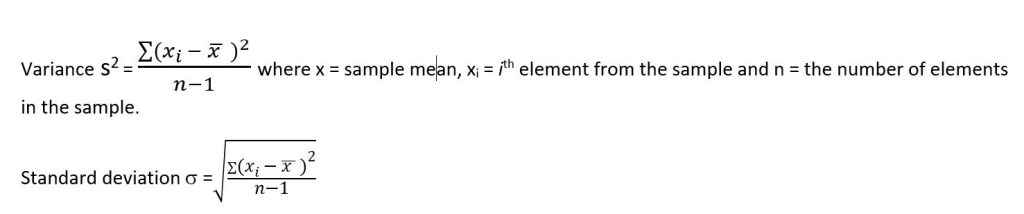
- Descriptive statistics for continuous variables
An example is a study conducted among 145 students where their height and weight were obtained. The summary statistics (a measure of central tendency and dispersion) have been presented below in table 3.2.
Table 3.2 Descriptive statistics for continuous variables
| Variable | Measures of central tendency | Measures of dispersion | ||||||
| Mean | Median | Mode | Variance | Standard deviation | Range | Minimum | Maximum | |
| Height (cm) | 169.8 | 169.0 | 164.0 | 60.4 | 7.8 | 89.0 | 151.0 | 190.0 |
| Weight (kg) | 68.9 | 66.0 | 60.0 | 163.1 | 12.8 | 74.0 | 46.0 | 120.0 |
- Descriptive statistics for categorical variables
Categorical variables are presented using frequencies and percentages or proportions. For example, a hypothetical scenario is a study on smoking history by gender in a population of 4609 people. Below is the summary statistic of the study (Table 3.3).
Table 3.3 Descriptive statistics for categorical variables
| Variable | Males | Females | ||
| N | Per cent | N | Per cent | |
| Smoking | ||||
| Smoker | 636 | 28.7% | 196 | 8.2% |
| Non-smoker | 1577 | 71.3% | 2200 | 91.8% |
| Total | 2213 | 2396 |
Normality of data
Before proceeding to inferential statistics, it is important to assess the normality of the data. A normality test evaluates whether or not a sample was selected from a normally distributed population.47 It is typically used to determine if the data used in the study has a normal distribution. Many statistical techniques, notably parametric tests, such as correlation, regression, t-tests, and ANOVA, are predicated on normal data distribution.47 There are several methods for assessing whether data are normally distributed. They include graphical or visual tests such as histograms and Q-Q probability plots and analytical tests such as the Shapiro-Wilk test and the Kolmogrorov-Smirnov test.47 The most useful visual method is visualizing the normality distribution via a histogram, as shown in Figure 3.12. On the other hand, the analytical tests (Shapiro-Wilk test and the Kolmogrorov-Smirnov) determine if the data distribution deviates considerably from the normal distribution by using criteria such as the p-value.47 If the p-value is < 0.05, the data is not normally distributed.47 These analytical tests can be conducted using statistical software like SPSS and R. However, when the sample size is > 30, the violation of the normality test is not an issue and the sample is considered to be normally distributed. According to the central limit theorem, in large samples of > 30 or 40, the sampling distribution is normal regardless of the shape of the data.47, 48 Normally distributed data are also known as parametric data, while non-normally distributed data are known as non-parametric data.
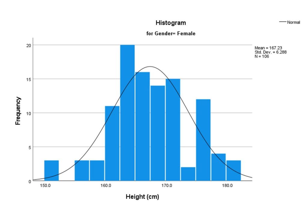
Table 3.4 Tests of normality for height by gender
| Tests of Normality | |||||||
| Height (cm) | Gender | Kolmogorov-Smirnov | Shapiro-Wilk | ||||
| Statistic | df | p-value (Sig.) | Statistic | df | p-value (Sig.) | ||
| Male | 0.059 | 39 | 0.200 | 0.983 | 39 | 0.814 | |
| Female | 0.082 | 106 | 0.076 | 0.981 | 106 | 0.146 | |
Inferential statistics
This statistical analysis involves the analysis of data from a sample to make inferences about the target population.45 The goal is to test hypotheses. Statistical techniques include parametric and non-parametric tests depending on the normality of the data.45 Conducting a statistical analysis requires choosing the right test to answer the research question.
Steps in a statistical test
The choice of the statistical test is based on the research question to be answered and the data. There are steps to take before choosing a test and conducting an analysis.49
- State the research question/aim
- State the null and alternative hypothesis
The null hypothesis states that there is no statistical difference exists between two variables or in a set of given observations. The alternative hypothesis contradicts the null and states that there is a statistical difference between the variables.
- Decide on a suitable statistical test based on the type of variables.
Is the data normally distributed? Are the variables continuous, discrete or categorical data? The identification of the data type will aid the appropriate selection of the right test.
- Specify the level of significance (α -for example, 0.05). The level of significance is the probability of rejecting the null hypothesis when the null is true. The hypothesis is tested by calculating the probability (P value) of observing a difference between the variables, and the value of p ranges from zero to one. The more common cut-off for statistical significance is 0.05. 50
- Conduct the statistical test analysis- calculate the p-value
- Make a statistical decision based on the findings
- p<0.05 leads to rejection of the null hypothesis
- p>0.05 leads to retention of the null hypothesis
- Interpret the results
In the next section, we have provided an overview of the statistical tests. The step-by-step conduct of the test using statistical software is beyond the scope of this book. We have provided the theoretical basis for the test. Other books, like Pallant’s SPSS survival manual: A step-by-step guide to data analysis using IBM SPSS, is a good resource if you wish to learn how to run the different tests.48
Types of Statistical tests
A distinction is always made based on the data type (categorical or numerical) and if the data is paired or unpaired. Paired data refers to data arising from the same individual at different time points, such as before and after or pre and post-test designs. In contrast, unpaired data are data from separate individuals. Inferential statistics can be grouped into the following categories:
- Comparing two categorical variables
- Comparing one numerical and one categorical variable
- o Two sample groups (one numerical variable and one categorical variable in two groups)
- o Three sample groups (one numerical variable and one categorical variable in three groups)
- Comparing two numerical variables
Comparing two categorical variables
Deciding on the choice of test with two categorical variables involves checking if the data is nominal or ordinal and paired versus unpaired. The figure below (Figure 3.13) shows a decision tree for categorical variables.
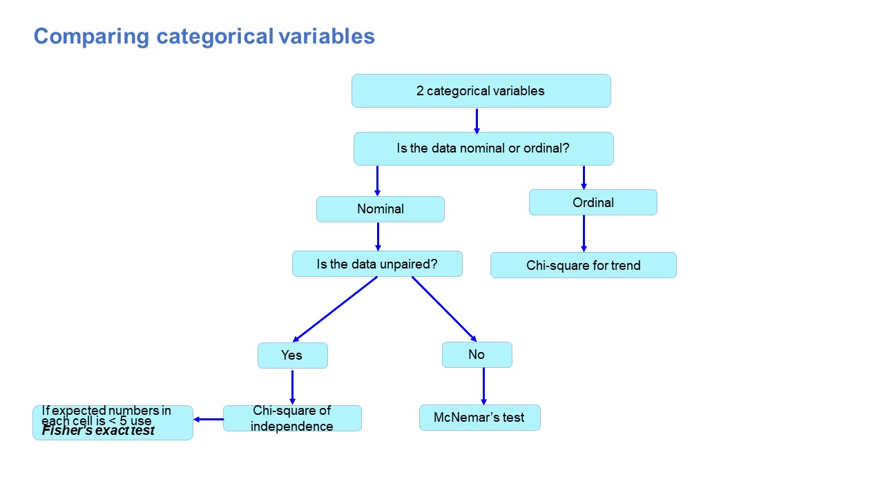
- Chi-square test of independence
The chi-square test of independence compares the distribution of two or more independent data sets.44 The chi-square value increases when the distributions are found to be increasingly similar, indicating a stronger relationship between them. A value of χ2 = 0 means that there is no relationship between the variables.44 There are preconditions for the Chi-square test, which include a sample size > 60, and the expected number in each field should not be less than 5. Fisher’s exact test is used if the conditions are not met.
- McNemar’s test
Unlike the Chi-square test, Mcnemar’s test is designed to assess if there is a difference between two related or paired groups (categorical variables).51
- Chi-square for trend
The chi-square test for trend tests the relationship between one variable that is binary and the other is ordered categorical.52 The test assesses whether the association between the variables follows a trend. For example, the association between the frequency of mouth rinse (once a week, twice a week and seven days a week) and the presence of dental gingivitis (yes vs no) can be assessed to observe a dose-response effect between mouth rinse usage and dental gingivitis.52
Tests involving one numerical and one categorical variable
The variables involved in this group of tests are one numerical variable and one categorical variable. These tests have two broad groups – two sample groups and three or more sample groups, as shown in Figures 3.14 and 3.15.
Two sample groups
The parametric two-sample group of tests (independent samples t-test and paired t-test) compare the means of the two samples. On the other hand, the non-parametric tests (Mann-Whitney U test and Wilcoxon Signed Rank test) compare medians of the samples.
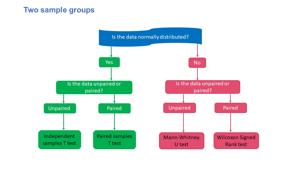
- Parametric: Independent samples T-test and Paired Samples t-test
The independent or unpaired t-test is used when the participants in both groups are independent of one another (those in the first group are distinct from those in the second group) and when the parameters are typically distributed and continuous.44 On the other hand, the paired t-test is used to test two paired sets of normally distributed continuous data. A paired test involves measuring the same item twice on each subject.44 For instance, you would wish to compare the differences in each subject’s heart rates before and after an exercise. The tests compare the mean values between the groups.
- Non-parametric: Mann-Whitney U test and Wilcoxon Signed Rank test
The nonparametric equivalents of the paired and independent sample t-tests are the Wilcoxon signed-rank test and the Mann-Whitney U test.44 These tests examine if the two data sets’ medians are equal and whether the sample sets are representative of the same population.44 They have less power than their parametric counterparts, as is the case with all nonparametric tests but can be applied to data that is not normally distributed or small samples.44
Three samples group
The t-tests and their non-parametric counterparts cannot be used for comparing three or more groups. Thus, three or more sample groups of the test are used. The parametric three samples group of tests are one-way ANOVA (Analysis of variance) and repeated measures ANOVA. In contrast, the non-parametric tests are the Kruskal-Wallis test and the Friedman test.
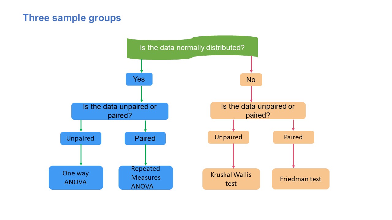
- Parametric: One-way ANOVA and Repeated measures ANOVA
ANOVA is used to determine whether there are appreciable differences between the means of three or more groups.45 Within-group and between-group variability are the two variances examined in a one-way ANOVA test. The repeated measures ANOVA examines whether the means of three or more groups are identical.45 When all the variables in a sample are tested under various circumstances or at various times, a repeated measure ANOVA is utilized.45 The dependent variable is measured repeatedly as the variables are determined from samples at various times. The data don’t conform to the ANOVA premise of independence; thus, using a typical ANOVA in this situation is inappropriate.45
- Non-parametric: Kuskal Wallis test and Friedman test
The non-parametric test to analyse variance is the Kruskal-Wallis test. It examines if the median values of three or more independent samples differ in any way.45 The test statistic is produced after the rank sums of the data values, which are ranked in ascending order. On the other hand, the Friedman test is the non-parametric test for comparing the differences between related samples. When the same parameter is assessed repeatedly or under different conditions on the same participants, the Friedman test can be used as an alternative to repeated measures ANOVA.45
Comparing two numerical variables
Pearson’s correlation and regression tests are used to compare two numerical variables.
- Pearson’s Correlation and Regression
Pearson’s correlation (r) indicates a relationship between two numerical variables assuming that the relationship is linear.53 This implies that for every unit rise or reduction in one variable, the other increases or decreases by a constant amount. The values of the correlation coefficient vary from -1 to + 1. Negative correlation coefficient values suggest a rise in one variable will lead to a fall in the other variable and vice versa.53 Positive correlation coefficient values indicate a propensity for one variable to rise or decrease in tandem with another. Pearson’s correlation also quantifies the strength of the relationship between the two variables. Correlation coefficient values close to zero suggest a weak linear relationship between two variables, whereas those close to -1 or +1 indicate a robust linear relationship between two variables.53 It is important to note that correlation does not imply causation. The Spearman rank correlation coefficient test (rs) is the nonparametric equivalent of the Pearson coefficient. It is useful when the conditions for calculating a meaningful r value cannot be satisfied and numerical data is being analysed.44
Regression measures the connection between two correlated variables. The variables are usually labelled as dependent or independent. An independent variable is a factor that influences a dependent variable (which can also be called an outcome).54 Regression analyses describe, estimate, predict and control the effect of one or more independent variables while investigating the relationship between the independent and dependent variables. 54 There are three common types of regression analyses – linear, logistic and multiple regression.54
- Linear regression examines the relationship between one continuous dependent and one continuous independent variable. For example, the effect of age on shoe size can be analysed using linear regression.54
- Logistic regression estimates an event’s likelihood with binary outcomes (present or absent). It involves one categorical dependent variable and two or more continuous or categorical predictor (independent) variables.54
- Multiple regression is an extension of simple linear regression and investigates one continuous dependent and two or more continuous independent variables.54
